Tunable lasers handbook phần 3 pps
Bạn đang xem bản rút gọn của tài liệu. Xem và tải ngay bản đầy đủ của tài liệu tại đây (1.12 MB, 50 trang )
84
Charles
Freed
r
Laser-Cavity Mirrors
7
(4.3~)
PFL
Detector
(Saturation
4
Resonance)
FIGURE
8
Graphic illustration
of
the
saturation resonance observed in
CO,
fluorescence at
4.3
pm.
Resonant interaction occurs
for
v
=
vo
(when
k
1’
=
0).
The
figure shows
an
internal absorption
cell within the laser cavity. External cells can also
be
used. (Reprinted with permission from
SooHoo
et
d.
[76].
0
1985
IEEE.)
In the initial experiments. a short gas cell with a total absorption path of
about 3 cm was placed inside the cavity of each stable
CO,
laser
[72]
with a
Brewster angle window separating the cell from the laser
g&
tube. Pure
CO,
gas at various low pressures was introduced inside the sample cell.
A
sapphire
window at the side of the sample cell allowed the observation of the 4.3-pm
spontaneous emission signal with a liquid-nitrogen-cooled InSb detector. The
detector element was about
1.5
cm from the path
of
the laser beam in the sample
cell.
To
reduce the broadband noise caused by background radiation. the detec-
tor placement was chosen to be at the center of curvature of a gold-coated spher-
ical mirror, which was internal
to
the gas absorption cell. The photograph
of
the
laser with which the standing-wave saturation resonance was first observed via
the fluorescence signal at
4.3
pm is shown in Fig.
9.
More than two orders
of
magnitude improvements in signal-to-noise ratios
(SNRs)
were subsequently
achieved with improved design low-pressure
CO,
stabilization cells external
to
the lasers
[73].
One example
of
such improved design is schematically shown in
Figure
10.
In the improved design, the low-pressure gas cell, the LN,-cooled radiation
collector, and the infrared
(IR)
detector are all integral partsbf one evacuated
housing assembly. This arrangement minimizes signal absorption by windows
and eliminates all other sources
of
absorption. Because of the vacuum enclo-
sure. diffusion of other gases into the low-pressure gas reference cell
is
almost
completely eliminated; therefore, the time period available for continuous use
of the reference gas cell is greatly increased and considerably less time has
to
be wasted
on
repumping and refilling procedures. One
LN,
fill can last at least
several days.
4
CO,
Isotope Lasers and Their Applications
85
FIGURE
9
Two-mirror stable laser with
short
intracavity cell.
This
laser
was
used
for
the first
demonstration
of
the standing-wave saturation resonance observed via the 4.3-pm fluorescence signal.
FIGURE
1
0
Schematic illustration
of
improved external
CO,
reference gas stabilization cell.
With the improved cells, significantly larger signal collection efficiency
was achieved simultaneously with a great reduction of noise due to background
radiation, which is the primary limit for high-quality InSb photovoltaic detec-
tors. We have evaluated and tested several large-area InSb detectors and deter-
mined that the LN,-cooled background greatly diminished
llf
noise in addition
to the expected reduction in white noise due to the lower temperature back-
ground radiation.
Figure
11
shows a typical recorder tracing
of
the observed 4.3-ym intensity
change as the laser frequency is tuned across the 10.59-ym
P(20)
line profile
86
Charles
Freed
fm=260Hz
r
=
0.1
aec
(single
pole)
16.4%
DIP
Ps1.75W;
PO
p
=
a034
Torr
FIGURE
1 1
Lamb-dip-like appearance
of
the resonant change in the 4.3-pm fluorescence. The
magnitude
of
the dip
is
16.4%
of
the 4.391 fluorescence signal. The pressure in the reference cell
was 0.034 Torr and the laser power into the cell was 1.75
W
in the
I-P(20)
transition.
A
frequency
dither rate
of
260
Hz was applied to the piezoelectric mirror tuner.
with a 0.034-Torr pressure of
12C160,
absorber gas. The standing-wave satura-
tion resonance appears in the form of a narrow resonant 16.4% “dip” in the 4.3-
pm signal intensity, which emanates from all the collisionally coupled rotational
levels in the entire (OOOl)+(OOO) band. The broad background curve is due to
the laser power variation as the frequency is swept within its oscillation band-
width. Because collision broadening in the
CO,
absorber is about 7.5 MHzRorr
FWHM
[72], in the limit of very low gas cell pressure the linewidth is deter-
mined primarily by power broadening and by the molecular transit time across
the diameter of the incident beam. The potentially great improvements in
SNR,
in reduced power and transit-time broadening, and in short-term laser stability
were the motivating factors that led to the choice of stabilizing cells external to
the laser’s optical cavity. The one disadvantage inherent with the use of external
stabilizing cells is that appropriate precautions must be taken to avoid optical
feedback into the lasers to be stabilized.
For frequency reference and long-term stabilization, it is convenient to
obtain the derivative of the 4.3-pm emission signal as a function of frequency.
This 4.3-pm signal derivative may be readily obtained by a small dithering of
the laser frequency as we slowly tune across the resonance in the vicinity of the
absorption-line center frequency. With the use of standard phase-sensitive detec-
tion techniques we can then obtain the 4.3-pm derivative signal to be used as a
frequency discriminator. Figure 12 shows such a 4.3-pm derivative signal as a
function of laser tuning near the center frequency of the 10.59-pm P(20) transi-
tion. The derivative signal in Fig. 12 was obtained by applying a f200-kHz fre-
quency modulation to the laser at a 260-Hz rate.
A
1.75-W portion of the laser’s
output was directed into a small external stabilization cell that was filled with
4
CO,
Isotope
Lasers
and
Their
Applications
87
S/N
=
-1000
Af
=
-f
200
kHz
tm
=
260
Hz
T
=
0.1
we
(ringla
pole)
Po
=
1.m
W;
P(20);
l0.6~
p
=
0.034
Torr
FIGURE
12
nance shown in Fig.
11.
SNR
-
1000,
Af
-
f200
kHz,
and
t
=
0.1
sec
(single pole).
Derivative signal at
4.3
pm
in the vicinity
of
the standing-wave saturation reso-
pure
CO,
to a pressure of 0.034 Torr at room temperature. It is a straightforward
procedure to line-center-stabilize a
CO,
laser through the use of the 4.3-pm
derivative signal as a frequency discriminant, in conjunction with a phase-sensi-
tive detector. Any deviation from the center frequency of the lasing transition
yields a positive or negative output voltage from the phase-sensitive detector.
This voltage is then utilized as a feedback signal in a servoloop to obtain the
long-term frequency stabilization of the laser output.
Figure 13 shows a block diagram of a two-channel heterodyne calibration
system. In the system, two small, low-pressure, room-temperature C0,-gas ref-
erence cells external to the lasers were used to line-center-stabilize two grating-
controlled stable lasers. The two-channel heterodyne system was used exten-
sively for the measurement and calibration of C0,-isotope laser transitions
[36,37].
Figure 14 shows the spectrum-analyzer display
of
a typical beat-note of the
system shown in Fig. 13. Note that the
SNR
is greater than
50
dB at the 24.4 GHz
beat frequency
of
the two laser transitions with the use of varactor photodiode
detection developed at
MIT
Lincoln Laboratory [74,75].
Figure 15 illustrates the time-domain frequency stability that we have rou-
tinely achieved with the two-channel heterodyne calibration system by using the
88
Charles
Freed
FIGURE
1
3
Block diagram
of
the two-channel line-center-stabilized C0,-isotope calibration
system.
In
the figure, wavy and solid lines denote optical and electrical paths, respectively. (Reprinted
with permission from Freed
[75].
0
1982
IEEE.)
-20
-30
52
dB
m^
-40
'D
0
9
-50
I
7
-60
-70
-80
4
+
200kHz
FIGURE
14
The 24.4104191-GHz beat note of a 16012CfSO laser I-P(l2) transition and a
l*C1602 laser
I-P(6)
transition. The power levels into the photodiode were 0.48 mW
for
the
16012C180 laser and 0.42 mW
for
the 12C160, laser. The second harmonic of the microwave local
oscillator was generated in the varactor photodiode. The intermediate-frequency noise bandwidth
of
the spectrum analyzer was set to
10
kHz.
4
CO,
Isotope Lasers
and
Their
Applications
89
I
I
I
I1111~
I
I
I
I I
Ill[
I
I
I I
Ill
10-10
M
=
50
h
-
d
g
10.11
:
2
A
HP
5061
CESIUM
u)
P
0
ATOMIC STANDARD
z
2
W
;
10-12
E
@
C02
SHORT-TERM STABILITY
0.01
0.1
1
.o
10
I00
SAMPLE
TIME,
T
(s)
FIGURE
1s
Time-domain frequency stability
of
the
2.6978618-GHz
beat note of the
'jCl30,
laser
i-Ri21)
transition and the
lTl6O0,
reference laser
I-P(?Oj
transition in the two-channel hetero-
dyne calibration system (Fig.
13)
with
the
4.3-pm
fluorescence stabilization technique
For
the sake
of
comparison. the stabilities
of
a cesium clock and short-term stabilities of individuai
CO,
lasers are
also
shown. Note that the frequencj stabilities of the
CO,
and the cesium-stabilized systems shown
are about the same and that the
CO,
radar has achieved short-term stabilities of at least tlbo
to
three
orders
of
magnitude better than those
of
microwave systems. (Reprinted with permission from
SooHoo
eral.
[76].
0
1981
IEEE.)
4.3-ym fluorescence stabilization technique
[56.76.77].
The solid and hollow
circles represent two separate measurement sequences of the Allan variance
of
the
frequency stability
Each measurement consisted of
M
=
50
consecutive samples for a sample time
duration (observation time) of
T
seconds. Figure
15
shows that we have achieved
OJT)
<?x
10-12
for
T-10
sec. Thus a frequency measurement precision
of
about
50
Hz
may be readily achieved within a few minutes.
90
Charles
Freed
The triangular symbols in Fig. 15 represent the frequency stability of a
Hewlett-Packard (HP) model
5061B
cesium atomic frequency standard, as spec-
ified in the HP catalog. Clearly, the frequency stabilities of the CO, and the
cesium-stabilized systems shown in Fig.
15
are about the same.
The two cross-circles in the lower left corner of Fig. 15 denote the upper
bound of the short-term frequency stabilities, as measured in the laboratory (Fig.
6) and determined from
CO,
radar returns at the Lincoln Laboratory Firepond
Facility
[56,58].
Note that the CO, radar has achieved short-term stabilities of at
least two to three orders of magnitude better than those of microwave systems.
Figure 16 shows the frequency reproducibility of the two-channel line-
center-stabilized
CO,
heterodyne calibration system. The figure contains a
so-
called drift run that was taken over a period
of
8.5
hours beginning at 1:OO
P.M.
[56,76,77].
The frequency-stability measurement apparatus was fully automatic;
it continued to take, compute, and record the beat-frequency data of the two line-
center stabilized
CO,
isotope lasers even at night. when
no
one was present in the
laboratory. Approxinlately every 100 sec the system printed
out
a data point that
represented the deviation from the
2.6976648-GHz
beat frequency, which was
'2C'602
I-P(Z0);
'3C'802
I-R(24);
T
=
10
s;
M
=
8
-2
E
31
-3
I
NOON
1
2
3
4
5
6
7
8
9
ELAPSED TIME
(h),
TIME
OF
DAY
FIGURE
16
Slow drifts in the 7.6978648-GHz beat frequency due to small frequency-offset-
ting zero-voltage variations of the electronics. The frequency deviations were caused
by
ambient
temperature variations.
The
beat note was derived from the
13C1800:
I-R(24)
and the
12C'602
I-P(Z0)
laser transitions.
An
obsemation time of
'I
=
10
sec and a sample size of
:21
=
8
were used for each
data point. (Reprinted with permission from
SooHoo
er
nl.
[76].
0
1985
IEEE.)
4
CO,
Isotope Lasers and Their Applications
91
averaged over
8.5
hours. The system used a measurement time of
T
=
10 sec and
A4
=
8
samples for each data point. yielding a measurement accuracy much better
than the approximately
f
1-kHz peak-frequency deviation observable in Fig. 16.
The frequency drift was most likely caused by small voltage-offset errors
in the phase-sensitive detector-driven servoamplifier outputs that controlled the
piezoelectrically tunable laser mirrors. Because
500
V
was required to tune the
laser one longitudinal mode spacing of
100
MHz, an output voltage error of
i2.5 mV
in
each channel was sufficient
to
cause the peak-frequency deviation
of
fl
kHz that was observed in Fig. 16. By monitoring the piezoelectric drive
voltage with the input to the lock-in amplifier terminated with a
50-SZ
load
(instead
of
connected to the InSb 4.3-ym fluorescence detector), we determined
that
slow
output-offset voltage drifts were the most probable cause of the
il-
kHz
frequency drifts observed in Fig. 16. It is important
to
note that no special
precautions were taken to protect either the lasers or the associated electronic
circuitry from temperature fluctuations in the laboratory. The temperature Wuc-
tuatians were substantial-plus
or
minus several degrees centigrade. Significant
improvements are possible with more up-to-date electronics and a temperature-
controlled environment.
Perhaps the greatest advantage of the 4.3-ym fluorescence stabilization
method
is
that it automatically provides a nearly perfect coincidence between the
lasing medium's gain profile and the line center of the saturable absorber, because
they both utilize the same molecule.
CO,.
Thus every
P
and
R
transition of the
(0001
j-[lOOO.
02@0],,,,
regular bands and the (Olll) [Ol@O, 0310],.,, hot bands
[78-811
may be line-center-locked with the same stabilization cell and gas
fill.
Furthermore, as illustrated in Fig.
8,
the saturation resonance is detected sepa-
rately at the 4.3-pm fluorescence band and not as a fractional change in the much
higher power laser radiation at
8.9
to
12.4
ym.
At
4.3 ym, InSb photovoltaic
detectors that can provide very high background-limited sensitivity are available,
However, it is absolutely imperative to realize that cryogenically cooled InSb
photovoltaic elements are extremely sensitive detectors of radiation far beyond
the 4.3-pm
CO,
fluorescence band. Thus, cryogenically cooled
IR-
bandpass fil-
ters and field-of-view
(FOV)
shields. which both spectrally and spatially match
the detector to the
CO,
gas volume emitting the 4.3-ym fluorescence radiation,
should be used. If this is not done. the detected radiation emanating from other
sources (ambient light, thermal radiation from laboratory personnel and equip-
ment, even electromagnetic emission from motors, transformers, and transmit-
ters) may completely swamp the desired
4.3-ym
fluorescence signal. This proce-
dure
is
a very familiar and standard technique utilized in virtually every sensitive
IR
detection apparatus; surprisingly, however, it was
only
belatedly realized
in
several very highly competent research laboratories. because the most commonly
used and least expensive general-purpose
IR
detectors are bought
in
a sealed-off
dewar and may not be easily retrofitted with a cryogenically cooled bandpass
fil-
ter and
FO'V
shield.
92
Charles
Freed
Additional precautionary measures should be taken in using the saturated
fluorescence signal. The Einstein coefficient for the upper lasing level
(0001)
is
about
200
to 300 sec-1 and. therefore, the modulation frequency must be slow
enough
so
that the molecules in the upper level have enough time to fluoresce
down to the ground state; here radiation trapping
[82,83]
of the 4.3-~m sponta-
neous emission (because
CO,
is a ground-state absorber) will show up as a vari-
ation of the relative phase between the reference modulation and the fluores-
cence signal as the pressure is vaned. The phase lag between the reference signal
and the molecular response would increase as the pressure increases because
there are more molecules to trap the 4.3-ym radiation and, therefore, hinder the
response. This phase lag will increase with increasing modulation frequency,
since the molecules will have less time to respond; thus, caution must be taken
when selecting the modulation frequency. A large phase lag will reduce the out-
put voltage (feedback signal) of the phase-sensitive detector; however, it will not
cause
a
shift in the instrumental zero
[76].
In addition to optimizing the frequency at which to modulate the laser, the
amplitude
of
the modulation (the frequency excursion due to the dithering) was
also considered in the experiments at Lincoln Laboratory
[76].
The modulation
amplitude must be large enough such that the fluorescence signal is detectable,
but the amplitude must be kept reasonably small to avoid all unnecessary para-
sitic amplitude modulation and nonlinearities in the piezoelectric response. in
order to avoid distorting the 4.3-pm Lorentzian. The maximum derivative signal
is obtained if the peak-to-peak frequency excursion equals
0.7
FWHM
of the
Lorentzian. But such a large excursion should be avoided in order to minimize
the likelihood of introducing asymmetries in the derivative signal. A compro-
mise modulation amplitude based on obtaining sufficient
SNR
for most
J
lines
was used. This modulation amplitude corresponded to a frequency deviation of
approximately
300
kHz peak-to-peak on a Lorentzian with an
FWHM
of about
1
MHz.
Experimental results indicated that the modulation frequency should be
kept well below
500
Hz.
At such low frequencies, InSb photovoltaic detectors
may have very high llfnoise unless operated at effectively zero dc bias voltage.
This may be best accomplished by a low-noise current mode preamplifier that is
matched to the dynamic impedance of the detector and is adjusted as close as
possible to zero dc bias across the detector (preferably less than
0.001
V).
There
are
other advantages of the 4.3-pm fluorescence stabilization; because
the fluorescence lifetime is long compared to the reorientating collision time at
the pressures typically employed in the measurements, the angular distribution
of the spontaneous emission is nearly isotropic. This reduces distortions of the
lineshape due to laser beam imperfections. Furthermore, only a relatively short
(3-
to 6-cm) fluorescing region is monitored, and the
CO,
absorption coefficient
is quite small
(-10-6
cm-1-Torr-1); this eliminates laser beam focusing effects
due to the spatial variation of the refractive index of the absorbing medium pro-
duced by the Gaussian laser beam profiles
[84,85].
Indeed, we have found no
4
CO,
Isotope
Lasers and Their Applications
93
significant change in the beat frequency after interchanging the two stabilizing
cells, which had very different internal geometries and volumes, and (within
the
frequency resolution of our system)
no
measurable effects due to imperfect
and/or slightly truncated TEMoo, beam profiles.
We have used external stabilizing cells with 2-cm clear apertures at the beam
entrance window. Inside the cell, the laser beam was turned back
on
itself (in
order to provide a standing wave) by means of a flat, totally reflecting mirror.
Slight misalignment of the return beam was used as a dispersion-independent
means
of
avoiding optical feedback. External stabilizing cells were used, instead
of
an
internal absorption cell within the laser cavity, in order to facilitate the opti-
mization of
SNIP,
in the 4.3-pm detection optics, independent of laser design con-
straints. External cells w-ere also easily portable and usable with
any
available
laser. The FWHM of the saturation resonance dip ranged from 700
kHz
to
1
or
2
MHz
as the pressure was varied from
10
to about
200
to 300 mTorr within the
relatively small (2-crn clear aperture) stabilizing cells employed in our experi-
ments.
By
using a 6.3-cm-diameter cell, 164-kHz RVHM saturation resonance
dips were reported by Kelly
[86].
Because the
FWHM
of the
CO,
saturation res-
onance due to pressure is about 7.5 kHz/mTorr. much of the lin&idth broaden-
ing
is
due to other causes such as power and transit-time broadening, second-
order Doppler shift. and recoil effects. More detailed discussions
of
these causes
can be found in
[76,112],
and in the literature on primary frequency standards but
any further consideration of these effects is well beyond the scope of this chapter.
The saturated
4.3-pm
fluorescence frequency stabilization method has been
recently extended to sequence band
CO,
lasers by Chou et
al.
[87,88]. The sequence
band transitions in
CO,
are designated
as
(000~)-[100(u-
1). 020
(u-
l)lI.*.
where
li
>
1
(u
=
1
defines the-regular bands discussed
in
this and previous sections of this
chapter). Sequence band lasers were intensively studied by Reid and Siemsen at the
NWC in Ottawa beginning in 1976
[89,90].
Figure
17
shows the sinnplified vibra-
tional energy-level diagram of the CO, and
N,
molecules, with solid-line
arrows
showing the
various
cw lasing bands observed
so
far. The dotted-line
arro\vs
show
the 43-pm fluorescence bands that were utilized for line-center stabilization
of
the
great multitude
of
individual lasing transitions.
Figure
17
clearly shows that for the (0002)-[1001,
0201],,,
first sequence
band transitions the laver laser levels are approximately 2300 crn-1 above those
of the regular band transitions and therefore the population densities of the first
sequence band laser levels are about four orders of magnitude less than in the
corresponding regular band laser levels. Chou
er al.
overcame this problem
by
using a heated longitudinal C07 absorption cell (L-cell) in which the 4.3-ym
fluorescence was monitored through a 3.3yrn bandpass filter in the direction of
the laser beam [87,88]. Due to the increased CO, temperature, photon trapping
[82,83,87]
was reduced. and by increasing the fluorescence collecting length
they increased the intensity of sequence band fluorescence
so
that
z.
good enough
SNR
was obtained at relatively low cell temperatures.
94
Charles
Freed
8000
6000
A
r
I
k
&
4000
W
a
3
2000
0
u=3
[I
1
1,03’1
I,
-
-
[I
220,0420],
z-
U=O
N2 GROUND
STATE
C02
GROUND
STATE
(00’0)
FIGURE
1
7
Simplified vibrational energy-level diagram
of
the
CO,
and
N2
molecules. The las-
ing bands are shown by solid-line
arrows.
The extra heavy
arrows
indicate lasing bands that were
only recently observed
[80.81].
The dotted-line
arrows
show the 1.3-pm fluorescence bands that
were used for line-center-frequency stabilization
of
the corresponding lasing transitions. (Reprinted
!&irh permission from Evenson
er
al.
[80].
Q
1994
IEEE.)
Although first demonstrated with
CO,
lasers, the frequency stabilization
technique utilizing the standing-wave saturation resonances via the intensity
changes observed in the spontaneous fluorescence (side) emission can be (and
has been) used with other laser systems as well (e.g.,
N,O)
[86].
This method of
frequency stabilization is particularly advantageous whenever the absorbing
transition belongs to a hot band with a weak absorption coefficient (such as
CO,
and
N,O).
Of course, saturable absorbers other than
CO,
(e.g.,
SF,,
OsO,)
can-and have been used with
CO,
lasers, but their use will not be discussed
here; the utilization of such absoibers requires the finding of fortuitous near
coincidences between each individual lasing transition and a suitable absorption
feature in the saturable absorber gas to be used. Indeed, just the preceding con-
siderations prompted the search for an alternate method of frequency stabiliza-
tion that could utilize the lasing molecules themselves as saturable absorbers. It
was this search for an alternate method
of
line-center stabilizing
of
the vast
multitude of potentially available lasing transitions in
CO,
lasers that finally led
Javan and Freed to the invention
[91]
and first demonstration
[48]
of the stand-
ing-wave saturation resonances in the
4.3-pm
spontaneous emission band
of
4
CO,
Isotope
Lasers and
Their
Applications
95
CO? and also the utilization of these narrow Doppler-free resonances for line-
center stabilization of all available regular and hot band CO, lasing transitions.
Since
its
first demonstration in 1970, this method of line-center stabilization has
attained worldwide use and became known as the
Freed-Javan
technique.
9.
ABSOLUTE FREQUENCIES
OF
REGULAR BAND LASING
TRANSITIONS IN NINE
CO,
ISOTOPIC
SPECIES
Through the use of optical heterodyne techniques [36,37,56,92-98], beat
frequencies between laser transitions of individually line-center-stabilized C0,-
isotope lasers in pairs can be generated and accurately measured. Measuremenis
of the difference frequencies are then used to calculate the band centers, rota-
tional constants, and transition frequencies by fitting the measured data to the
standard formula for the term values [31,36-38.931 as given here:
The first systematic measurement and really accurate determination of the absolute
frequencies and vibrational-rotational constants
of
the regular band 12C1601 laser
transitions was accomplished by Petersen
et
al.
of the
NBS
in 1973 [93.$5].
In
these initial measurements Petersen
et
al.
used 30 adjacent pairs of 12C160, laser
lines in the
10.4-pm
regular band and
26
adjacent pairs in the 9.3-pm regular
band. The lasing transitions were generated by
tm
o
grating-controlled 12C16Q7
lasers, which were line-center-stabilized using the standing-wave saturation reso:
nances observed in the 4.3-pm fluorescence band, and the 3240 63-GHz beat fre-
quencies were detected and measured using LHe temperature Josephson junctions.
These measurements, together with the absolute frequencies
of
the
10.18-pm
I-
R(30) and 9.33-pm
11-R(
10)
W160,
transitions as determined relative to the
pn-
mary cesium frequency standard at the
NBS
in Boulder, Colorado, by Evenson
et
al.
in
1973 [94], reduced the uncertainties in existing vibrational-rotational con-
stants
[92]
20
to
30 times and the additional rotational constant
H,
was determined
€or the first time
with
a statistically significant accuracy.
Concurrent with the ongoing work mith 13C1601 lasers at the
NBS,
we at
MIT
Lincoln
Laboratory concentrated our effort
on
measuring the rare
CO,
isotopic
species using LN,-cooled HgCdTe varactor photodiodes [74.75] and-the
two-
channel line-center-stabilized CO,-isotope calibration system illustrated in
Fig.
13
and described in Sec.
8.
In
the initial phase of the MIT Lincoln Laboratory
work,
the band centers. rotational constants. absolute frequencies, and vacuum
nave
96
Charles
Freed
numbers for
12C1607,
W16O
2’
12C180,,
W18O
2’
W160180,
14C1607.
and
14C180,
were simultaneousl; computed from 390 beat frequency measurements between
pairs
of
adjacent (0001)-[ 1000,
0200],~,,
band
C02
laser transitions. The input
data included the 56 beat frequencies measured between adjacent
12C1601
rota-
tional lines by Petersen
et
a/.
[93], and the absolute frequencies
of
the 10.18ym
I-
R(30) and 9.33-ym 11-R(10)
12C160,
transitions determined by Evenson
et
al.
[94]
relative to the primary cesium standard. These initial results for the seven
CO,
iso-
topic species listed were published by Freed
et
al.
in 1980 [36].
In 1983 Petersen
et
al.
published
[99]
improved vibrational-rotational con-
stants and absolute frequency tables for the regular bands of
12C160,.
These new
results obtained at the
NBS
in Boulder, Colorado, were based
on
new beat fre-
quency measurements, including high-J and across-the-band center measure-
ments, and yielded about a factor of 10 better frequency tables.
In
addition,
some specific
13C1602
lines were also measured with reduced uncertainties. The
new results of Petersen
et
a/.
[99] yielded a more precise determination of the
absolute frequency (relative to the primary cesium standard)
of
the
12C160,
I-
R(30) line, with an absolute uncertainty of 3.1 kHz. This uncertainty of 3.1
kHz
became the principal limit for the uncertainties in the frequency tables for the
absolute frequencies of regular band lasing transitions in nine
C02
isotopic
species, published by Bradley
et
al.
in 1986 [37]. The data and results published
in this paper represented the final phase and outcome of the isotopic
CO,
laser
frequency-calibration work that had begun at
MIT
Lincoln Laboratory more than
a decade earlier. This final
CO,
isotope frequency calibration work represented
significant improvement over previous results for the following reasons:
1. We have included in our database the most recent measurements on
13C160,
regular band transitions that Petersen
et al.
published [99]; their more
precise-measurement of the I-R(30) line absolute frequency, and the beat fre-
quencies of their widely spaced lines [99] was included in our database as shown
in Table 1.
2.
We have extended our previous measurements, particularly of
lC1601
to
higher
J
values, and have made the first measurements of
12C170,
-
&d
3. We have improved our instrumentation and measurement techniques. and
thus have been able to measure pressure shifts in
CO,
laser lines with a more
sophisticated two-channel line-center-stabilized calibration system (which is
described in the next section).
4.
We have recognized deficiencies in our earlier weighting of measure-
ments, and have become familiar with the use of resistant statistical procedures
for minimizing the effects of “outliers.”
As
a result of the preceding changes, the number of beat frequency measurements
has increased
to
915, the number
of
isotopic species has increased to nine, and
the precision
of
predicted frequencies has increased by an order of magnitude.
13C160180.
TAN€
1
Absolute Fieyuency
and
Four-Frequency Beat Measui-enients
of
Petersen
ct
a!.
[W]“
MBArmRBD
NOMINAL CALCDLATBD
MEMURED-
FRBQUEblcy
STD.DBV.
FRBQUEMCY
CALCOLATBD
0.0000
626
R
I(30) 29442483.3191 3.1D-03 29442483.3191
FOUR-FREQUENCY BEATS PBTERSBN
BT
AL.
I1
MBA8uRHD
NOMINAL CALCOLATBD
MBAmJRBD
-
RBLATIVB
FRBQUEMCIBS STD.DBV.
PRgooBIICIBS CALCOLATBD DBVIATION
2.626
R
I(12)
-
626
R
II(10)
22941.9100
2.5D-03
22941.9093
0.0007
0.21
-
636 P I(50)
2.626 P I(34)
-
636
P
II(28) 15433.4420 2.5~-03 15433.4428
-0.0008
-0.33
-
636 P
I(50)
-
“Reprinted
with
penni\hi
from
Brqdley
(31
(//,
1371.
0
19x6
EEE.
98
Charles
Freed
Figure
18
graphically illustrates the frequency and wavelength domain of
the nine
CO?
isotopic species that have been measured to date. The
14C160,
extends the wavelength range to well beyond 12
pm;
13C180,
transitions can
reach below
9
ym. We have fitted the data obtained from the
915
beat frequency
measurements and the ones shown in Table
1
to the polynomial formula for term
values described in Eq.
(1
8).
The molecular constants derived from the fit. the
frequencies. wave numbers (using
c
=
299 792
458
m/s), and standard deviations
predicted are shown in Tables
2
through
10
for the regular bands of the isotopic
species
of
CO,
that we measured (out of
18
possible isotopic combinations). We
have printed the molecular constants with more figures than their standard devia-
tions warrant
so
that those who wish to use the constants to generate frequencies
will find agreement with our predicted frequencies. We
may
also remark that
some linear combinations
of
molecular constants [e&.
B(OOl)-B(I)]
are better
determined than any
of
the constants individually. With each constant
is
printed
an ordinal number; these numbers are used to designate the
rows
and columns of
Il-R
Il-P
I-R
I-P
Il-R
Il-P
I-R
I-P
WAVE NUMBER
(an-'l
I
I
I
I
I
I
I
1
9.0
9.6
10.0
10.5 11.0
11.5
12.0 12.5
WAVELENGTH
(p)
FIGURE
1
8
(Reprinted with permission from Freed
[56].)
Frequency
and
wavelength domain
of
lasing transitions in nine
co,
isotopes
4
CO,
Isotope Lasers
and
Their Applications
9
the variance-covariance matrix, the lower triangle of which is shown in Table
XI1 of the original paper
[37],
but is not reproduced here.
The horizontal lines drawn in the frequency tables denote the highest and
lowest
J
lines within which beat frequency measurements were used in the data
for computer fitting.
As
always. the frequency values outside the measured
regions should be used with the greatest caution, and the computed standard
deviations for such lines should be considered as only a rough guide.
The original paper
[37]
also contains the
915
beat frequency measurements
and their nominal standard deviations that constituted the input
to
our computa-
tions. These data, which are designated as Files
1
through
50
in Table I1 of
[37],
will be useful to those who wish to derive better molecular constants and more
accurate frequency determinations as additional beat frequency measurements
and more precise intercomparisons of CO, lasing transitions with the prirnar:
frequency standard (cesium at the present) become available.
The frequencies predicted in Tables
2
through
10
show, for the most accurate
lines, standard deviations that are an order of magnitude smaller than those in
[36]
and are principally limited by the uncertainty in the single absolute frequency mea-
surement. We believe that these standard deviations are reasonable estimates of the
uncertainties of their respective frequencies, and that our molecular constants and
predicted frequencies are the best currently available for the
CO,
isotopic species,
and are as good as any that can be extracted from the available data.
In
our opinion,
they are suitable (with appropriate care about sequence and hot bands
[78-81.
89,90,10&103])
for use as secondarp standards at the indicated level of precision.
Higher precision (by perhaps two orders of magnitude) in the CQ, comparisons
could be attained by application of techniques developed in
[76],
whiih are summa-
rized in the next section. but for more precise absolute frequencies. this would need
to be accompanied by a similarly precise comparison with the cesium standard,
During the preparation of the manuscript for this chapter I became aware
of
some very recent mork on
CO,
laser line calibration that was carried out at the
Time and Frequency Division
if
NIST in Boulder, Colorado.
I
am grateful to
Dr.
K,
hl.
Evenson for providing me with a very recent reprint
[80]
and three addi-
tional manuscripts prior
to
their publication
[38,81,88].
The outcome of this nev.
work
will
result in improved molecular constants and frequencies for the
CQ,
laser and mill be very briefly summarized next.
In
May
1994,
Evenson
et al.
reported
[80]
the first observation of laser tran-
sitions in the (O0~1~ [11~0.0310],, 9-pm hot band of
12C1607.
This band
is
iden-
tified
bj
an
extra
heavy solid
arrow
in the vibrational energy level diagram
of
Fig.
17,
nhich was reproduced from
[XO].
These transitions. together with the
(001
1) [111O.
03101,
lower frequency hot band transitions that were previously
measured
by
Whitford
et
al.
[78] and by Petersen
et
al.
[79] were incorporated
into a new database by
Maki
et
al.
[38].
Altogether they included 84 hot band
transitions and also
12
higher
J
value regular band
W1607
transitions that were
not measured by Bradley
er
a1
[37].
From the database provided in Bradley
er
o!.
100
Charles
Freed
TABLE
2
Molecular
Constants
and
Frequencies Calculated for
626a
NUMBER
SYMBOL
1
V(OO1-I)
=
2
V(OO1-11)
=
16 12 16
OCO
LINE FREQUENCY
(rnZ
1
P( 60) 2707
7607.5077
P(581 2714
6404.4578
2721 4396.1809
2728 1588.8741
2734 7988.4259
2741 3600.4235
2747 8430.1601
2754 2482.6413
2760 5762.5914
2766 8274.4599
2773 0022.4271
2779 1010.4094
2785 1242.0651
2791 0720.7986
2796 9449.7656
2802 7431.8776
2808 4669.8055
2814 1165.9839
CONSTANTS
(MHZ
1
2.880 001 382 455 D+07
3.188 996 017 636 D+07
1.160
620
695
034 D+04
1.169
756 942
611 D+04
1.170 636
464 791 D+04
3.988
109 863 0-03
3.445
940 508 D-03
4.711
559 114 D-03
0.481 534 D-09
5.625
110
D-09
7.066
300
D-09
-0.96
936 D-14
1.06 816 D-14
-4.31 765 D-14
BAND
I
STD.
DEV
.
VAC.WAVE
NO.
(MHZ
1
(CM-1)
0.0246 903.2117 6484
0.0154 905.5065 8408
0.0097
0.0064
0.0049
0.0043
0.0040
0.0038
0.0037
0.0036
0.0036
0.0036
0.0035
0.0035
0.0035
0.0035
0.0035
0.0035
907.7745 4384
910.0158 5084
912.2307 0148
914.4192 8214
916.5817 6938
918.7183 3017
920.8291 2210
922.9142 9359
924.9739 8407
927.0083 2419
929.0174 3596
931.0014 3295
932.9604 2043
934.8944 9550
936.8037 4726
938.6882 5692
STD.DEV.
(MHZ
1
3.6D-03
3.7D-03
2.3D-05
2.5D-05
2.4D-05
3.2D-08
3.3D-08
3.3D-08
1.9D-11
1.
ED-11
1.
ED-11
3.5D-15
3.3D-15
3.2D-15
(continues)
4
CO,
Isotope
Lasers
and
Their
Applications
10
TABLE
2
(conrinuedj
LINE
FREQUKNCY
(MHZ
1
2819 6922.6147
2825 1941.6703
2830 6224.8967
2835 9773.8165
2841 2589.7314
2846 4673.7246
2851 6026.6628
2856 6649.1983
2861 6541.7701
2866 5704.6061
2871 4137.7235
2876 1840.9300
2880 8813.8246
2883 2026.2225
2887 7902.4412
2892 3046.4336
2896 7457.0695
2901 1133.0097
2905 4072.7058
2909 6274.3988
2913 7736.1185
2917 8455.6817
2921 8430.6909
2925 7658.5324
2929 6136.3?40
2933 3861.1629
2937 0829.6231
2940 7038.2525
2944 2483.3197
2947 7160.8609
2951 1066.6762
2954 4196.3256
2957 6545.1250
2960 8108.1417
2963 8880.1900
2966 8855.8259
2969 8029.3420
2972 6394.7621
2975 3945.8353
BAND
I
fcontinur
STD.
DEV
.
WHZ)
0.0036
0.0036
0.0036
0.0036
0.0035
0.0035
0.0035
0.0035
0.0035
0
0036
0.0036
vi)
VAC.WAVE
NO.
(CM-1)
940.5480 9793
942.3833 3608
944.1940 2961
945.9802 2931
947.7419 7860
949.4793 1361
951.1922 6324
952.8808 4927
954.5450 8632
956.1849 8202
957.8005 3691
0.0035
0.0035
0.0035
0.0034
0.0034
0.0033
0.0033
0.0032
0.0032
0.0032
0.0031
0.0031
0
0031
0.0031
0.0031
0.0032
0.0033
0.0033
0.0034
0.0035
0.0035
0.0036
0.0045
966.2503 6076
967.7072 3331
969.1395 4739
910.5472 4435
971.9302 5845
973.2885 1688
974.6219 3965
975.9304 3960
977,2139 2224
978.4722 8575
979.7054 2084
980.9132 1071
982.0955 3089
983.2522 4916
984.3832 2542
985.4883
1157
986.5673 5137
987.6201 8028
988.6466 2533
989.6465 0491
990.6196 2866
991.5657 9723
992.4848 0211
2978 0676.0297
0.0070 993.3764 2542
2980 6578.5263
0.0117 994.2404 3971
2983 1646.2123 0.0193 995.0766
0771
2985
5871.6737 0.0307
995.8846 8212
BAND
I1
P(601
3014 3456.0702 0.0172 1005.4774 6515
pi58j 3021 2223.6949
o.oiio
1007.7713 0607
8
P(56) 3028 032 .120 0.0428 03
P(54) 3034 7743.7465 0.0051 1012.2917 6841
P(52) 3041 4481.1364 0.0042 1014.5178 8812
P(50) 3048 0527.0251 0.0039 1016.7209 4183
coririnues)
102
Charles
Freed
TABLE
2
lconfinuedJ
LINE
FREQUENCY
p(48) 3054 5874.3277
P(46) 3061 0516.1462
P(44) 3067 4445.7759
P(42) 3073 7656.7119
~(40)
3080
0142.6555
~(38) 3086 1897.5199
~(36) 3092 2915.4360
p(34) 3098 3190.7583
~(32) 3104 2718.0700
P
(30)
3110 1492.1877
P
(28) 3115 9508.1671
~(26) 3121 6761.3064
P(24) 3127 3247.1518
P(22) 3132 8961.5006
P(20)
3138
3900.4054
P(18) 3143 8060.1774
P(16) 3149 1437.3897
P (14) 3154 4028.8804
P(12) 3159 5831.7547
p(10) 3164 6843.3878
p(
8)
3169 7061.4264
P( 6) 3174 6483.7910
P(
4) 3179 5108.6771
(MHZ
1
BAND
I1
(continued)
STD.
DEV
.
VAC.WAVE
NO.
(MHZ
1
0.0038
0.0039
0.0039
0.0039
0.0039
0.0038
0.0038
0.0038
0.0038
0.0037
0.0037
0.0037
0.0038
0.0038
0.0038
0.0037
0.0037
0.0037
0.0037
0.0037
0.0037
0.0037
0.0037
(CM-1)
1018.9006 9322
1021.0569 1219
1023.1893 7509
1025.2978 6496
1027.3821 7169
1029.4420 9223
1031.4774 3083
1033.4879 9917
1035.4736 1655
1037.4341 1009
1039.3693 1486
1041.2790 7402
1043.1632 3901
1045.0216 6964
1046.8542 3425
1048.6608 0978
1050.4412 8194
1052.1955 4524
1053.9235 0313
1055.6250 6805
1057.3001 6151
1058.9487 1415
1060.5706 6576
pi 2j 3184 2934.5560 0.0037 1062.1659 6536
V(
0)
3188 9960.1764 0.0037 1063.7345 7121
R(
0)
3191 3172.5743 0.0037 1064.5088 5347
R( 2) 3195 8996.0672 0.0036 1066.0373 6066
R( 4) 3200 4017.3872 0.0036 1067.5391 1025
R( 6) 3204 8236.2544 0.0036
R(
8)
3209 1652.6660 0.0036
R(10) 3213 4266.8953 0.0036
R(12) 3217 6079.4907 0.0036
R(16)
3225
7303.3400 0.0037
R(18)
3229
6717.0518 0.0037
R(20)
3233
5334.0411
0.0038
R(22)
3237
3156.2043 0.0039
R(24)
3241
0185.7000 0.0039
R(26)
3244
6424.9456 0.0039
R(28)
3248
1876.6140 0.0040
R(30)
3251
6543.6298 0.0040
R(32)
3255
0429.1653 0.0039
R(34)
3258
3536.6360 0.0039
R(36)
3261
5869.6965 0.0039
R(38)
3264
7432.2354
0.0038
R(40)
3267
8228.3702 0.0038
R(42)
3270
8262.4421 0.0038
R(44)
3273
7539.0104 0.0038
R(46)
3276
6062.8469 0.0039
~(14) 3221 7091.2743 0.0037
R (48) 3279
3838.9297
0.0043
R (50)
3282 0872.4368
0.0055
R (52) 3284
7168.7402 0.0081
R(54)
328?
2733.3987 0.0127
R(56)
3289
7572.1515 0.0199
1069.0140 9289
1070.4623
0849
1071.8837 6618
1073.2784
8423
1074.6464
9008
1075.9878
2021
1077.3025
2013
1078.5906 4423
1079.8522
5580
1081.0874
2682
1082.2962
3794
1083.4787 7831
1084.6351 4549
1085.7654
4528
1086.8697
9163
1087.9483 0644
1089.0011
1941
1090.0283
6790
1091.0301
9670
1092.0067
5790
1092.9582 1067
1093.8847
2107
1094.7864
6180
1095.6636
1206
1096.5163
5728
1097.3448 8889
R158) 3292 1690.9108
0.0305
1098.1494 0411
"Reproduced
with
permission from Bradley
era/.
[37].
0
1986IEEE.
4
CO,
Isotope Lasers and Their Applications
103
TABLE
3
Molecular Constants and Frequencies Calculated for
636"
NUMBER
SYMBOL
15 V(OO1-I)
=
16 V(OO1-11)
=
17 B(001)
=
-
18
BCI)
-
19 B(II)
-
-
26 L(001)
=
27 L(1)
-
28 L(II)
-
-
-
16 13 16
OCO
LINE
FREQUENCY
(MHZ
1
P(60) 2572
0428.2139
P(58) 2578
4672.4669
P(56) 2584
8281.2715
P (54) 2591
1259.2641
2597 3610.8059
2603 5339.9930
2609 6450.6662
2615 6946.4203
2621 6830.6129
2627 6106.3727
2633 4776.6070
2639 2844.0093
2645 0311.0659
2650 7180.0624
2656 3453.0895
2661 9132.0488
2667 4218.6576
2672 8714.4542
CONSTANTS
(MHZ
1
2.738 379 258 341 D+07
3.050 865 923 183 D+07
1.161 016 490 148 D+04
1.168
344
168 872 D+04
1.171
936
491 647 D+04
3.984
584 753 D-03
3.604 500 429 D-03
4.747
234 294 D-03
0.495 934 D-09
6.338
964 D-09
8.203 342 D-09
-2.29 763 D-14
5.77 901 D-14
-7.93 174 D-14
BAND
I
STD. DEV
.
VAC.WAVE
NO.
(MHZ
1
(CM-1)
0.1461 857.9411 3653
0.0893 860.0840 9414
0.0506 862.2058 5547
0.0254 864.3065 7519
0.0104 866.3863 9875
0.0046
0.0060
0.0071
0.0069
0.0062
0.0055
0.0050
0.0048
0.0041
0.0047
0.0046
0.0045
0.0044
868.4454 6280
870.4838 9544
872.5018 1658
874.4993 3824
876.4165 6475
878.4335 9311
880.3705
1317
882.2874 0784
884.1843 5338
886.0614 1951
881.9186 6968
889.7561 6117
891.5739 4527
STD. DEV
.
(MHZ
1
4.5D-03
4.6D-03
1
a
1D-04
1.2D-04
1
e
2D-04
1
40-07
1 5D-07
1 5D-07
?
=
2D-11
7 6D-11
7
ED-11
1
3D-14
1.4D-14
1
~
5D-14
(continues)
104
Charles Freed
TABLE
3
(continlied)
LINE
PRBOUENCY
(MHZ
1
2678 2620.8016
2683 5938.8924
2688 8669.7518
2694 0814.2416
2699 2373,0626
2704 3346.7581
2709 3735.7157
2714 3540.1700
2719 2760.2041
BAND
I
continue^
STD.
DEV
.
(MHZ
1
0.0045
0.0046
0.0048
0.0049
0.0051
0.0051
0.0051
0.0051
0.0050
!f)
VAC.WAVE
NO.
(CM-1)
893.3720 6747
895.1505 6754
896.9094 7969
898.6488 3264
900.3686 4979
902.0689 4925
903.7497 4396
905.4110 4173
907.0528 4534
P( 6)
2724 1395.7513 0.0049
908.6751 5257
P( 4) 2728
9446.3964
0.0048 910.2779
5624
P( 2)
2733 6912.3769
0.0046 911.8612
4425
V(
0)
2738
3792.5834
0.0045 913.4249
9962
R(
0)
2740
7012.8973
0.0044
914.1995 4592
R( 2) 2745
3013.4681
0.0042
915.7339 5979
(
4)
2749 8426.5523 0.0041 917,2487 7725
R(
6) 2754
3251.1293
0.0039 918.7439
6418
0.0038
0.0037
0.0037
0.0037
0.0037
0.0037
0.0037
0.0037
0.0036
0.0036
0.0036
0.0036
0.0036
0.0037
0.0037
0.0037
0.0038
0.0039
0.0047
0.0075
0.0138
0.0251
0.0432
0.0708
0.1112
0.1688
BAND
I1
0.2555
0.1690
0.1079
0.0660
0.0383
0.0208
0.0108
0.0060
0.0046
2758 7486.0315
2763 1129.9444
2767 4181.4046
2771 6638.7995
2775 8500.3648
2779 9764.1836
2784 0428.1832
2788 0490.1338
2791 9947.6446
2795 8798.1618
2799 7038.9645
2803 4667.1610
2807 1679.6853
2810 8073.2921
2814 3844.5522
2817 8989.8473
2821 3505.3647
2824 7387.0908
2828 0630.8053
2831 3232.0738
2834 5186.2410
2837 6488.4223
2840 7133.4961
2843 7116.0949
2846 6430.5956
2849 5071.1098
2872 9056.6508
2887 0077.7355
2879 9935.4314
2893 9475.6922
2900 8121.5973
2907 6007.9210
2914 3127.3153
2920 9472.6220
2927 5036.8795
920.2194 8169
921.6752 8592
923.1113 2806
924.5275 5431
925.9239 0583
927.3003 1866
928.6567 2369
929.9930 4651
931.3092 0741
932.6051 2117
933.8806 9704
935.1358 3858
936.3704 4349
937.5844 0354
938.7776 0434
939.9499 2520
941.1012 3893
942.2314 1167
943.3403 0262
944.4277 6388
945.4936 4017
946.5377 6855
947.5599 7818
948.5600 9002
949.5379 1651
950.4932 6124
958.2981 7876
960.6624 4039
963.0021 3581
965.3170 0248
967.6067 8340
969.8712 2741
972.1100
8942
974.3231 3064
976.5101 1886
(continues)
4
CO,
Isotope Lasers and Their Applications
105
TABLE
3
(continued)
LINE
BREQUENCY
(MHZ
1
2933 9813.3301
2940 3795.4270
2946 6976.8409
2952 9351.4664
2959 0913.4284
2965 1657.0881
2971 1577.0489
2977 0668.1613
2982 8925.5288
298% 6344.5126
2994 2920.7360
2999 8650.0890
3005 3528.7321
3010 7553.1003
3016 0719.9062
3021 3026.1432
BAND
11
(conrinuedi
STD.
DEV
.
VAC.WAVE
NO.
(MHZ
1
(CM-1)
0.0042 978.6708
2867
0.0040 980.8050
4170
0.0037
982.9125 4682
0.0036
984,9931 4037
0.0035
987.0466 2638
0.0034
989.0728 1677
0.0034 991.0715
3152
0.0035 993.0425
9887
0.0037
994.9858 5548
0.0039
996.9011 4661
0.0043
998.7883 2629
0.0046
1000.6472 5741
0.0048
1002.4778 1190
0.0050
1004.2798 7085
0.0050
1006.0533 2460
0.0050
1007.7980 7286
P(l0j 3026 4469.0880 0.0050 1009.5140 2480
P(
E)
3031 5046 .3034 0.0049 1011.2010 9911
P(
6)
3036 4755.6398 0.0048 1012.8592 2409
P( 4) 3041 3595.2374 0.0048 1014.4883 3771
P(
2) 3046 1563.5271 0.0047 1016.0883 8762
V(
0)
3050 8659.2318 0.0046 1017.6593 3124
R(
0)
3053 1879.5457 0.0046 1018.4338 7754
R(
2) 3057 7664.6183 0.0045 1019.9611 0317
R(
4)
3062 2575.1933 0.0044 1021.4591 5870
R(
6)
3066 6611.0178
R(
8)
3070
9772.1308
R(10)
3075 2058.8624
R(12) 3079 3471.8321
R(14)
3083 4011.9476
RI16)
3087 3680.4026
R(18)
3091 2478.6741
R(20) 3095 0408.5204
R(22) 3098 7471.9774
R(24) 3102 3671.3557
R(26) 3105 9009.2365
R
(28) 3109 3488.4681
R(30)
3112 7112.1611
R(34) 3119
1806.6581
R(36)
3122
2884.9526
R(38) 3125
3122.6789
R(40) 3128
2524.1847
R(42) 3131
1094.0483
R(44) 3133
8837.0719
R(46) 3136
5758.2755
R(48) 3139
1862.8900
R(50)
3141
7156.3502
R(52) 3144
1644.2875
R154) 3146
5332.5230
R(56) 3148
8227.0596
RI58)
3151
0334.0742
R
(32
j
3115 9883.6840
0.0042
0.0041
0.0041
0,0040
0.0040
0.0040
0.0040
0.0040
0.0040
0.0039
0
a
0039
0.0040
0.0040
0.0040
0.0041
0.0041
0.0043
0.0047
0.0054
0.0071
0.0112
0.0193
0.0332
0.0555
0.0892
0.1386
0.2089
1022.9280 3569
1024.3677 3546
1025.7782 6899
1027.1596 5697
1028.5119 2966
1029.8351 2689
1031.1292 9793
1032.3945 0141
1033.6308 0526
1034.8382 8655
1036.0170 3137
1037.1671 3474
1038.2887 0042
1039.3818 4075
1040.4466 7655
1041.4833 3687
1042.4919 5885
1043.4726 8752
1044.4256 7559
1045.3510 8324
1046.2490 7794
1047.1198 3415
1047.9635 3316
1048.7803 6283
1049.5705 1732
1050.3341 9685
1051.0716 0749
"Reproduced
wi;h
permission
from
Bradley
er
al.
[37].
0
1986
IEEE.
106
Charles Freed
TABLE
4
Molecular Constants and Frequencies Calculated for
628"
16 12 18
OCO
NUMBER
SYMBOL
29
V(OO1-I)
=
2.896
801
233 901
D+07
30 V(O0l-11)
=
3.215
835 064
653 D+07
31 B(001)
=
1.095 102 264 016 D+04
1.104 772 438 281 D+04
32 B(1)
-
1.103 600 443 963 D+04
33 B(I1)
-
-
-
34 D(OO1)
=
3.550 909 355 D-03
3.064 795 497 D-03
35 D(1)
-
4.096 110 317 D-03
36 D(I1)
-
-
-
40 L(OO1)
=
41 L(1)
-
42 L(I1)
-
-
-
FREQUENCY
(MHZ
1
2729 6371.2432
2733 0160.6851
2736 3739.9515
2739 7109.7225
2743 0270.6628
2746 3223.4212
2749 5968.6313
2752 8506.9114
2756 0838.8646
2759 2965.0793
2762 4886.1287
2765 6602.5715
2768 8114.9518
2771 9423.7991
2775 0529.6287
2778 1432.9417
2781 2134.2250
2784 2633.9515
BAND
I
STD.DEV.
(MHZ
1
2.7312
2.2947
1.9182
1.5948
1.3182
1.0828
0.8834
0.7153
0.5746
0.4575
0.3606
0.2812
0.2165
0.1644
0.1229
0.0901
0.0647
0.0453
0.074 060 D-09
2.945 673 D-09
4.419 934 D-09
5.56 243
D-14
7.69 066 D-14
64.89
108
D-14
VAC.WAVE NO.
(CM-1)
910.5089 3759
911.6360 3206
912.7561 1582
913.8692 1156
914.9753 4147
916.0745 2717
917.1667 8981
918.2521 5000
919.3306 2788
920.4022 4305
921.4670 1465
922.5249 6130
923.5761 0116
924.6204 5190
925.6580 3069
926.6888 5425
927.7129 3883
928.7303 0020
STD
.
DEV
.
(MHZ
1
1.OD-02
2.3D-02
2.8D-04
3.OD-04
2.8D-04
5.2D-07
5.5D-07
6.3D-07
4.OD-10
4.2D-10
6.20-10
1.1D-13
1.1D-13
2.1D-13
~
(continues)
4
CO,
Isotope Lasers and Their Applications
107
TABLE
4
(continued)
BAND
I
(conrinued~
LINE
FREQUENCY
STD.
DEV
.
VAC.WAVE NO.
(MHZ)
(MHZ
1
(CM-1)
PI421 2787 2932.5802 0.0308 929.7409 5366
P(41) 2790 3030.5565 0.0203 930.7449 1409
P(40) 2793 2928.3119 0.0130 931.7421 9586
P(39) 2796 2626.2643
2799 2124.8184
2802 1424.3652
2805 0525.2826
2807 9427.9351
2810 8132.6743
2813 6639.8385
2816 4949.7533
2819 3062.7312
2822 0979.0720
2824 8699.0627
2827 6222.9778
2830 3551.0789
2833 0683.6152
2835 7620.8235
2838 4362.9282
2841 0910.1411
2843 7262.6619
2846 3420.6781
2848 9384.3647
2851 5153.8849
2854 0729.3895
28515 6111.0174
2859 1298.8955
2861 6293.1385
2864 1093.8494
2866 5701.1190
2869 0115.0266
2871 4335.6392
2873 8363.0123
2876 2197.1895
2878 5838.2025
2880 9286.0713
2883 2540.8044
2885 5602.3982
2887 8470.8376
2890 1146.0958
2892 3628.1341
2894 5916.9025
2896 8012.3390
2898
9914.3701
2901 1622.9105
2903 3137.8634
2905 4459.1202
2907 5586.5606
2909 6520.0529
2911 7259.4532
2913 7804.6065
0
10084
0.0059
0.0050
0.0048
0.0047
0.0045
0
0044
0.0043
0
0042
0.0041
0.0041
0.0041
0.0041
0.0041
0.0040
0.0040
0.0040
0.0039
0.0039
0.0040
0.0040
0.0039
0.0039
0.0039
0.0039
0.0039
0.0040
0.0041
0.0044
0.0047
0.0052
0.0057
0.0063
0.0069
0.0075
0.0081
0.0087
0.0093
0.0097
0
*
0101
0.0104
0.0106
0.
0108
0.0108
0.0108
0.0107
0.0105
0.0103
932.7328 1292
933.7167 7877
934.6941 0645
935.6648 0857
936.6288 9729
937.5863 8432
938.5372 8096
939.4815 9808
940.4193 4608
941.3505 3498
942.2751 7434
943.1932 7332
944.1048 4065
945.0098 8464
945.9084 1320
946.8004 3379
947.6859 5350
948.5649 7897
949.4375 1647
950.3035 7184
951.1631 5050
952.0162 5751
952.8628 9749
953.7030 7466
954.5367 9287
955.3640 5553
956.1848 6570
956.9992 2600
957.8071 3867
958.6086 0557
959.4036 2814
960.1922 0745
960.9743 4417
961.7500 3857
962.5192 9054
963.2820 9957
964.0384 6476
964.7883 8484
965.5318 5813
966.2688 8256
966.9994 5567
967.7235 7464
968.4412 3622
969.1524 3679
969,8571 7235
970.5554 3848
971.2472 3042
971.9325 4296
f
conrinuesJ
108
Charles Freed
TABLE
4 (continued)
LINE
FREQUENCY
(MHZ
1
2915 8155.3456
2917 8311.4918
2919 8272.8546
2921 8039.2319
2923 7610.4096
2925 6986.1619
2927 6166.2511
2929 5150.4278
2931 3938.4306
2933 2529.9861
2935 0924.8091
2936 9122.6024
2938 7123.0568
2940 4925.8509
2942 2530.6513
2943 9937.1125
2945 7144.8766
2947 4153.5738
2949 0962.8216
2950 7572.2255
2952 3981.3785
2954 0189.8609
2955 6197.2409
2957 2003.0737
2958 7606.9022
2960 3008.2564
2961 8206.6535
2963 3201.5979
2964 7992.5812
2966 2579.0817
2967 6960.5648
2969 1136.4828
2970 5106.2746
2971 8869.3657
2973 2425.1684
2974 5773.0814
2975 8912.4896
2977 1842.7644
2978 4563.2633
2979 7073.3299
2980 9372.2936
2982 1459.4700
2983 3334.1601
2984 4995.6509
2985 6443.2145
2986 7676.1087
2987 8693.5765
2988 9494.8460
2990 0079.1304
2991 0445.6275
2992 0593.5203
2993 0521.9760
BAND
I
(contin14
STD
.
DEV
.
(MHZ
1
0.0100
0.0096
0.0093
0.0089
0.0084
0.0080
0.0075
fed)
VAC.WAVE
NO.
(a-1)
972.6113 7055
973.2837 0722
973.9495 4661
974.6088 8199
975.2617 0620
975.9080 1173
976.5477 9064
0.0071 977.1810 3461
0.0066 977.8077 3493
0.0062
0.0057
0.0053
0.0050
0.0047
0.0044
0.0043
0.0041
0.0041
0.0040
0.0040
0.0039
0.0039
0.0039
0.0040
0.0042
0.0044
0.0047
0.0049
0.0052
0.0058
0.0074
0.0109
978.4278 8247
979.0414 6772
979.6484 8076
980.2489 1129
980.8427 4858
981.4299 8152
982.0105 9856
982.5845 8779
983.1519 3686
983.7126 3301
984.2666 6309
984.8140 1352
985.3546 7029
985.8886 1901
986.4158 4485
986.9363 3254
987.4500 6642
987.9570 3038
988.4572 0788
988.9505 8198
989.4371 3526
989.9168 4990
990.3897 0763
0.0168 990.8556 8972
0.0256 991.3147 7703
0.0381
0.0549
0.0772
0.1060
0.1428
0.1892
0.2469
0.3181
0.4052
0.5108
0.6381
0.7903
0.9714
1.1856
1.4377
1.7331
2.0776
2.4777
991.7669 4994
992.2121 8839
992.6504 7187
993.0817 7941
993.5060 8958
993,9233 8048
994.3336 2975
994.7368 1456
995.1329 1159
995.5218 9705
995.9037 4667
996.2784 3569
996.6459 3886
997.0062 3042
997.3592 8415
997.7050 7327
998.0435 7054
998.3747 4817
(continues)