Multiresolution Signal Decomposition Transforms, Subbands, and Wavelets phần 7 potx
Bạn đang xem bản rút gọn của tài liệu. Xem và tải ngay bản đầy đủ của tài liệu tại đây (2.71 MB, 52 trang )
4.10.
ALIASING
ENERGY
IN
MULTIRESOLUTION DECOMPOSITION
311
4-20
2
Figure
4.10 (continued)
312
CHAPTER
4,
FILTER
BANK
FAMILIES:
DESIGN
Figure 4.11:
(a)
Hierarchical decimation/interpolation
branch
arid
(b) its
equiva-
lent.
The
advantage
of
this analysis
in a
lossless
M-band
filter
bank structure
is its
ability
to
decompose
the
signal energy into
a
kind
of
time-frequency plane.
We
can
express
the
decomposed signal energy
of
branches
or
subbands
in
the form of
an
energy matrix
defined
as
(Akansu
and
Caglar, 1992)
Each
row of the
matrix
E
represents
one of the
bands
or
channels
in the
filter
bank
and the
columns correspond
to the
distributions
of
subband
energies
in
frequency.
The
energy matrices
of the
8-band
DCT, 8-band
(3-level)
hierarchical
filter
banks with
a
6-tap
Biriomial-QMF
(BQMF),
and the
most regular
wavelet
4.10.
ALIASING ENERGY
IN
MULTIRESOLUTION
DECOMPOSITION
318
filter
(MRWF)
(Daubechies)
for an
AR(1)
source with
p =
0.95
follow:
EDCT
—
EBQMF
-
EMRWF
—
~
6.6824
0.1511
0.0345
0.0158
0.0176
0.0065
0.0053
0.0053
"
7.1720
0.0567
0.0258
0.0042
0.0196
0.0019
0.0045
0.0020
"
7.1611
0.0589
0.0262
0.0043
0.0196
0.0020
0.0047
0.0020
0.1211
0.1881
0.0136
0.0032
0.0032
0.0012
0.0004
0.0002
0.0567
0.1987
0.0025
0.0014
0.0019
0.0061
0.0001
0.0001
0.0589
0.1956
0.0028
0.0018
0.0020
0.0064
0.0001
0.0001
0.0280
0.1511
0.0569
0.0050
0.0016
0.0065
0.0001
0.0000
0.0014
0.0567
0.0640
0.0025
0.0001
0.0019
0.0014
0.0001
0.0018
0.0589
0.0628
0.0028
0.0001
0.0020
0.0017
0.0001
0.0157
0.0265
0.0136
0.0279
0.0032
0.0022
0.0004
0.0000
0.0005
0.0258
0.0025
0.0295
0.0013
0.0046
0.0001
0.0001
0.0006
0.0262
0.0028
0.0291
0.0014
0.0047
0.0001
0.0001
0.0132
0.0113
0.0345
0.0051
0.0176
0.0026
0.0053
0.0000
0.0001
0.0005
0.0258
0.0025
0.0223
0.0013
0.0045
0.0001
0.0001
0.0006
0.0262
0.0028
0.0221
0.0014
0.0047
0.0001
0.0157
0.0091
0.0078
0.0032
0.0032
0.0132
0.0033
0.0002
0.0005
0.0014
0.0042
0.0014
0.0013
0.0167
0.0020
0.0001
0.0006
0.0017
0.0043
0.0018
0.0014
0.0164
0.0020
0.0001
0.0280
0.0113
0.0046
0.0158
0.0016
0.0026
0.0118
0.0053
0.0014
0.0005
0.0061
0.0042
0.0001
0.0013
0.0162
0.0020
0.0018
0.0006
0.0064
0.0043
0.0001
0.0014
0.0160
0.0020
0.1211
1
0.0265
0.0078
0.0061
0.0032
0.0022
0.0033
0.0155
0.0567
"
0.0258
0.0042
0.0196
0.0019
0.0045
0.0020
0.0220
0.0589
"
0.0262
0.0043
0.0196
0.0020
0.0047
0.0020
0.0218
We
can
easily
extend
this
analysis
to any
branch
in a
tree
structure,
as
shown
in
Fig.
4.11
(a).
We can
obtain
an
equivalent structure
by
shifting
the
antialiasing
niters
to the
left
of the
decimator
and the
interpolating
filter
to the
right
of the
up-sampler
as
shown
in
Fig.
4.11(b).
The
extension
is now
obvious.
4.10.2 Nonaliasing Energy Ratio
The
energy compaction measure
GTC
does
not
consider
the
distribution
of the
band energies
in
frequency. Therefore
the
aliasing portion
of the
band energy
is
treated
no
differently
than
the
nonaliasing component. This
fact
becomes
im-
portant
particularly when
all the
analysis
subband
signals
are not
used
for the
reconstruction
or
whenever
the
aliasing cancellation
in the
reconstructed signal
is
not
perfectly performed because
of the
available bits
for
coding.
From Eqs. (4.78)
and
(4.79),
we
define
the
nonaliasing energy
ratio
(NER)
of
314
CHAPTER
4.
FILTER BANK
FAMILIES:
DESIGN
an
M-band
orthonormal
decomposition technique
as
where
the
numerator term
is the sum of the
nonaliasing terms
of the
band
energies.
The
ideal
filter
bank yields
NER=1
for any M as the
upper bound
of
this measure
for
any
arbitrary input signal.
4.11
GTC
an(
i
NER
Performance
We
consider
4-,
6-,
8-tap
Binomial-QMFs
in a
hierarchical
filter
bank structure
as
well
as the
8-tap
Smith-Barnwell
and
6-tap most regular orthonormal wavelet
filters,
and the
4-,
6-,
8-tap
optimal
PR-QMFs
along with
the
ideal filter banks
for
performance
comparison. Additionally,
2 x 2, 4 x 4, and
8x8
discrete cosine,
dis-
crete sine,
Walsh-Hadamard,
and
modified
Hermite transforms
are
considered
for
comparison purposes.
The GTC
and
NER
performance
of
these
different
decom-
position
tools
are
calculated
by
computer simulations
for an
AR(1) source model.
Table
4.15
displays
GTC and NER
performance
of the
techniques considered with
M
=
2,4,8.
It is
well
known
that
the
aliasing energies become annoying, particularly
at low
bit
rate image coding applications.
The
analysis provided
in
this
section explains
objectively some
of the
reasons
behind
this
observation. Although
the
ratio
of the
aliasing energies over
the
whole signal energy
may
appear
negligible,
the
misplaced
aliasing energy components
of
bands
may be
locally
significant
in
frequency
and
cause subjective performance degradation.
While larger
M
indicates better coding performance
by the GTC
measure,
it is
known
that
larger size transforms
do not
provide
better
subjective image coding
performance.
The
causes
of
this undesired behavior have been mentioned
in the
literature
as
intercoefficient
or
interband energy leakages,
bad
time localization,
etc
The NER
measure indicates
that
the
larger
M
values yield degraded perfor-
mance
for the
finite
duration
transform
bases
and the
source models considered.
This trend
is
consistent with those experimental performance results reported
in
the
literature. This measure
is
therefore
complementary
to
GTC:
which
does
not
consider
aliasing.
4.12.
QUANTIZATION EFFECTS
IN
FILTER BANKS
315
DOT
DST
MHT
WHT
Binomial-QMF
(4
tap)
Binomial-QMF
(6
tap)
Binomial-QMF
(8
tap)
Smith-Barnwell
(
8tap)
Most
regular
(6
tap)
Optimal
QMF (8
tap)*
Optimal
QMF (8
tap)**
Optimal
QMF (6
tap)*
Optimal
QMF (6
tap)**
Optimal
QMF (4
tap)*
Optimal
QMF (4
tap)**
Ideal
filter
bank
M=2
G
TC
(NEK)
3.2026
(0.9756)
3.2026 (0.9756)
3.2026
(0.9756)
3.2026
(0.9756)
3.6426
(0.9880)
3.7588
(0.9911)
3.8109 (0.9927)
3.8391
(0.9937)
3.7447
(0.9908)
3.8566 (0.9943)
3.8530
(0.9944)
3.7962
(0.9923)
3.7936
(0.9924)
3.6527 (0.9883)
3.6525
(0.9883)
3.946 (1.000)
M=4
G
TC
(NER)
5.7151
(0.9372)
3.9106
(0.8532)
3.7577
(0.8311)
5.2173 (0.9356)
6.4322
(0.9663)
6.7665 (0.9744)
6.9076
(0.9784)
6.9786 (0.9813)
6.7255
(0.9734)
7.0111
(0.9831)
6.9899 (0.9834)
6.8624
(0.9776)
6.8471
(0.9777)
6.4659 (0.9671)
6.4662
(0.9672)
7.230 (1.000)
M=8
GTC
(NER)
7.6316 (0.8767)
4.8774 (0.7298)
4.4121 (0.5953)
6.2319 (0.8687)
8.0149 (0.9260)
8.5293 (0.9427)
8.7431 (0.9513)
8.8489 (0.9577)
8.4652
(0.9406)
8.8863
(0.9615)
8.8454 (0.9623)
8.6721 (0.9497)
8.6438 (0.9503)
8.0693 (0.9278)
8.0700
(0.9280)
9.160 (1.000)
*This
optimal
QMF is
based
on
energy compaction.
**This
optimal
QMF is
based
on
minimized aliasing energy.
Table 4.15: Performance
of
several orthonormal signal decomposition techniques
for
AR(1),
p —
0.95 source.
4.12
Quantization
Effects
in
Filter
Banks
A
prime purpose
of
subband
filter
banks
is the
attainment
of
data
rate
compres-
sion
through
the use of
pdf-optimized quantizers
and
optimum
bit
allocation
for
each subband signal.
Yet
scant consideration
had
been given
to the
effect
of
coding
errors
due to
quantization. Early studies
by
Westerink
et
al.
(1992)
and
Vanden-
dorpe (1991) were
followed
by a
series
of
papers
by
Haddad
and his
colleagues,
Kovacevic
(1993), Gosse
and
Duhamel (1997),
and
others.
This section provides
a
direct
focus
on
modeling, analysis,
and
optimum design
of
quantized
filter
banks.
It is
abstracted
from
Haddad
and
Park (1995).
We
review
the
gain-plus-additive noise model
for the
pdf-optimized quantizer
advanced
by
Jayant
and
Noll (1984). Then
we
embed this model
in the
time-
domain
filter
bank representation
of
Section 3.5.5
to
provide
an
M-band
quanti-
zation
model amenable
to
analysis. This
is
followed
by a
description
of an
optimum
316
CHAPTER
4.
FILTER
BANK
FAMILIES:
DESIGN
two-band
filter
design which incorporates quantization error
effects
in the
design
methodology.
4.12.1
Equivalent Noise Model
The
quantizer studied
in
Section 2.2.2
is
shown
in
Pig.
4.12(a).
We
assume
that
the
random variable input
x has a
known probability density
function
(pdf)
with
zero
mean.
If
this quantizer
is
pdf-optirnized,
the
quantization error
.? is
zero
mean
and
orthogonal
to the
quantizer output
x
(Prob.2.9),
i.e.,
But
the
quantization error
x is
correlated with
the
input
so
that
the
variance
of
the
quantization
is
(Prob. 4.24)
where
a
2
refers
to the
variance
of the
respective zero mean signals. Note
that
for
the
optimum quantizer,
the
output signal variance
is
less
than
that
of the
input.
Hence
the
simple input-independent additive noise model
is
only
an
approximation
to the
noise
in the
pdf-optirnized
quantizer.
Figure 4.12:
(a)
pdf-optimized quantizer;
(b)
equivalent noise model.
Figure
4.12(b)
shows
a
gain-plus-additive noise representation which
is to
model
the
quantizer.
In
this model,
we can
impose
the
conditions
in Eq.
(4.82)
and
force
the
input
x and
additive noise
r to be
uncorrelated.
The
model param-
eters
are
gain
a and
variance
of.
With
x
—
ax + r, the
uncorrelated requirement
becomes
4.12.
QUANTIZATION EFFECTS
IN
FILTER BANKS
317
Equating
cr|
in
these
last
two
equations gives
one
condition.
Next,
we
equate
E{xx}
for
model
and
quantizer. From
the
model,
and for the
quantizer,
These
last
two
equations provide
the
second
constraint.
Solving
all
these gives
For the
model,
r and x are
uncorrelated
and the
gain
a.
and
variance
a^,
are
input-signal dependent.
Figure 4.13:
/3(R),
a(R)
versus
R for
AR(1) Gaussian input
at
p=0.95.
From
rate
distortion theory (Berger 1971),
the
quantization error variance
<r|
for
the
pdf-optimized
quantizer
is
818
CHAPTER
4.
FILTER BANK
FAMILIES:
DESIGN
The
parameter
(3(R)
in Eq.
(4.89)
depends only
on the pdf of the
unit variance
signal
being quantized
and on
J?,,
the
number
of
bits assigned
to the
quantizer.
It
does
not
depend
on the
autocorrelation
of the
input signal. Earlier approaches
treated
(3(R)
as a
constant
for a
particular pdf.
We
show
the
plot
of
(3
versus
R
for
a
Gaussian input
in
Fig. 4.13. Jayant
and
Noll reported
{3=2,7
for a
Gaussian
input,
the
asymptotic value indicated
by the
dashed line
in
Fig.
4.13.
From Eqs.
(4.88)
and
(4.89)
the
nonlinear gain
a can be
evaluated
as
Figure
4.13 also shows
a vs R
using
Eq.
(4.90).
As R
gets
large,
j3
approaches
its
asymptotic value,
and a
approaches unity. Thus,
the
gain-plus additive noise
model
parameters
a and
d^
are
determined once
R and the
signal
pdf are
specified.
Note
that
a
different
plot
and
different
asymptotic value result
for
differing
signal
pdfs.
4.12.2
Quantization Model
for
M-Band
Codec
The
maximally decimated
M-band
filter
bank with
the
bank
of
pdf-optimized
quantizers
and a
bank
of
scalar compensators (dotted lines)
are
shown
in
Fig.
4.14(a).
Each quantizer
is
represented
by its
equivalent noise model,
and the
analysis
and
synthesis banks
by the
equivalent polyphase structures. This gives
the
equivalent representation
of
Fig.
4.14(b),
which,
in
turn,
is
depicted
by the
vector-matrix equivalent structure
of
Fig.
4.14(c).
Thus,
by
moving
the
samplers
to the
left
and
right
of the filter
banks,
and
focusing
on the
slow-clock-rate
signals,
the
system
to be
analyzed
is
time-invariant,
but
nonlinear because
of the
presence
of
the
signal dependent gain matrix
A.
By
construction
the
vectors
t>[n]
and
r[n]
are
uricorrelated,
and A, S are
diag-
onal gain
and
compensation matrices, respectively, where
This representation
well
now
permits
us to
calculate explicitly
the
total
mean
square quantization error
in the
reconstructed output
in
terms
of
analysis
and
syn-
thesis
filter
coefficients,
the
input signal autocorrelation,
the
scalar compensators.
and
implicitly
in
terms
of the bit
allocation
for
each band.
4.12.
QUANTIZATION EFFECTS
IN
FILTER BANKS
319
Figure 4.14:
(a)
M-band
filter
bank structure with compensators,
(b)
polyphase
equivalent
structure,
(c)
vector-matrix equivalent structure.
320
CHAPTER
4.
FILTER
BANK
FAMILIES:
DESIGN
We
define
the
total
quantization error
as the
difference
where
the
subscript
"o"
implies
the
system without quantizers
and
compensators.
From Fig.
4.14(c)
we see
that
where
B
-
S
-
/, and
V(z)
=
H
p
(z)£(z)
and
C(z)
=
G'
p
(z)B,
T>(z)
=
Q'
p
(z)S.
We
note
that
v(n)
and
r(n)
are
uncorrelated
by
construction.
For
a
time-invariant system with
M x 1
input vector
x and
output vector
y,
we
define
M x M
power spectral density (PSD)
and
correlation matrices
as
Using
these
definitions
and the
fact
that
v(n)
and
r(n)
are
uncorrelated,
we can
calculate
the PSD
S
nqnq
(z]
and
covariance
R
nq
n
q
[fn\
for the
quantization error
r)
q
(n).
It is
straightforward
to
show (Prob. 4.24) that
where
C(z]
«-»
Ck
and
T>(z)
+-*
D^
are Z
transform pairs.
At fc=0,
this becomes
From
Fig.
4.14(b),
we can
demonstrate
that
R
rm
(o]
is the
covariance
of the
Mth
block
output vector
4.12.
QUANTIZATION
EFFECTS
IN
FILTER BANKS
Consequently,
321
Note
that
this
is
cyclostationary;
the
covariance matrix
of the
next block
of M
outputs
will
also equal
/^[O].
Each block
of M
output samples
will
thus have
same
sum of
variances.
We
take
the MS
value
of the
output
as the
average
of the
diagonal elements
of Eq.
(4.101),
Similarly,
if we
define
y
q
(ri)
as the
quantization error
in the
reconstructed output
then
the
total mean square quantization error (MSE)
at the
system
output
is
Next,
by
substituting
Eq.
(4.99)
into
Eq.
(4.104),
we
obtain
The first
term,
<rj,
of Eq.
(4.105)
is the
component
of the MSE due to the
nonlinear
gain
matrix
A and
compensation matrix
S.
The
second term
a^
accounts
for the
322
CHAPTER
4.
FILTER
BANK
FAMILIES:
DESIGN
additive
fictitious
random noise
r(n).
These terms
<rj,
<r^
are
called
the
signal
distortion
and
random noise components
of the
MSE, respectively.
Under
PR
constraints,
<jj
measures
the
deviation
from
perfect reconstruction
due to the
quantizer
and
compensator. This decomposition
of the
total
MSE
enables
us
to
analyze each component error separately. This
is the
main theoretical
consequence
of
the
gain-plus-additive noise quantizer model where
the
signals
v(n)
and
random
noise
r(n)
are
uncorrelated.
The MSE in Eq.
(4.105)
can be
written
in an
explicit closed
form
time-domain
expression
in
te;rms
of the
analysis
and
synthesis
filter
coefficients.
This
is
achieved
by
expanding
the
polyphase
coefficient
matrices
in
terms
of the
synthesis
filter
coefficients
via
and
substituting into
Eq.
(4.105).
The
results
are
rather messy
and are not
pre-
sented here.
The
interested reader
can
refer
to the
reference
for
details.
The
last
step
In our
formulation requires
a
further breakdown
of
R
vv
[m]
in Eq.
(4.105).
Prom
Fig.
4.14(a)
R
ViVj
[m]
can be
represented
as
By
defining
the
correlation
function
pji(m)
—
hi(m)
*
hj(-rri).
we
have
This concludes
the
formulation
of the
output
MSE in
terms
of the
analy-
sis/synthesis
filter
coefficients
/ij(n),
gi(ri),
the
input autocorrelation
function
RXX[™}->
the
nonlinear gain
c^,
and
compensator
Si.
Some simplifying assumptions
on
R^k)
can be
argued. First,
we
note
that
the
decimated signals
('t^(n)}
occupy
frequency
bands
that
can be
made
to
overlap
slightly.
Hence,
{vi(n}}
and
{VJ(H
+
m)}
tend
to be
weakly correlated.
The
random
errors
{n(n)}
due to
each quantizer are,
by
design,
uncorrelated with
the
respective
{vi(n}}.
Therefore,
as a
simplifying assumption
we can say
that
.12.
UANTIZATION
EFFECTS
IN
FILTER BANKS
823
E[ri(n}rj(n
j
r-m)}
~
0.
This makes
Rrr[n}
a
diagonal matrix. Next,
it is
often
true
that
the
quantization error
for a
given signal swing
(as
measured
by
crjj
sweeps
over
several quantization levels. When this
is
true,
E[ri(n}ri(n
+
m)]
= of
,<S(m).
Then,
the
random component
of
reduces
to a
simpler
form
but
a^
remains messy.
From
the
foregoing,
several observations regarding compensators
can be
noted:
(i)
By
setting
Si=l,
we
have
no
compensation
and
a\
in Eq.
(4.105),
and
of
in
Eq.
(4.109)
constitute
the MSE in the
uncompensated structure.
As we
shall
see in
the
next section,
5^=1
is the
optimized selection when paraunitary
PR
constraints
are
imposed
on the
non-quantized system.
(ii)
By
choosing
Si
=
1/c^,
the
"null compensation,"
we can
eliminate com-
pletely
the
signal distortion term
o~§,
leaving only
the
noise term
(iii)
However, this solution
is not
optimal
at the
stated operating conditions.
The
quantizer gain
c^
< 1 and Eq.
(4.110) show
that
we can
expect
a
larger
random
component than
that
of the
uncompensated structure.
In
fact,
for the
uncompensated
structure, this random component
is
dominant. Increasing this
component
by the
null condition
is
decidedly
not
optimal.
(iv)
However, when
the
input statistics change
from
nominal values,
the
null
compensation
is
found
to be
superior
to the
"optimal" one, which
is, in
fact,
optimal only
at the
nominal values
of p. In
this account,
we
minimize
the
total
MSE
by
minimizing
jointly
the sum of
o\
and
o\
subject
to
defined
PR
constraints.
4.12.3 Optimal
Design
of
Bit-Constrained,
pdf-Optimized
Filter
Banks
The
design problem
is the
determination
of the
optimal
FIR
filter
coefficients,
compensators,
and
integer
bit
allocation
that
minimize
the MSE
subject
to
con-
straints
of filter
length, average
bit
rate,
and PR in the
absence
of
quantizers,
for
an
input signal with
a
given autocorrelation
function.
324
CHAPTER
4.
FILTER BANK
FAMILIES:
DESIGN
For
the
paraimitary
case,
the
orthogonality properties eliminate
the
cross-
correlation between analysis channels, which
is
implicit
in the
crj
component
of
Eq.
(4.105).
The
MSB
in
this case reduces
to
It is now
easy
to
show
that
the
optimized compensator
for
this
paraunitary
condi-
tion
is
s\
— 1.
Then
the
uncompensated system
is
optimal
for the
pdf-optimized
paraunitarjr
FB.
(On the
other hand,
si
=
1 is not
optimal
for the
biorthogona)
structure because
of the
cross-correlation between analysis channels.)
Sample designs
and
simulations
for a
six-coefficient
paraunitary two-band
structure
for an
AR(1) input with
p —
0.95
are
shown
in
Table 4.13.
MSE
refers
to the
theoretical calculations
and
MSE
s
j
m
,
the
simulation results. Table 4.13
demonstrates
that
the
optimal
filter
coefficients
are
quite insensitive
to
changes
in
the
average
bit
rate
R and in
input correlation
p.
Figure
4.15(a)
shows explicitly
the
distortion
and
random components
of the
total MSE.
The
simulation results
closely
match
the
theoretical ones.
The
random noise
cr^
is
clearly
the
dominant
component
of the
MSE. Figure
4.15(b)
compares
the
optimally compensated with
the
null compensated
(si —
l/cti)
paraunitary systems designed
for p
—
0.95.
The
null
compensated
is
more robust
for
changing input statistics
and
performs
better
than
the fixed
optimally compensated
one
when
p
changes
from
its
design
value
of
p
=
0.95.
Similar designs
and
simulations were executed
for the
biorthogonal two-band
case with equal length
(6
taps) analysis
and
synthesis
filters. For the
same operat-
ing
conditions,
the
biorthogonal structure
is
superior
to the
paraunitary
in
terms
of
the
output MSE. However,
the
biorthogonal
filter
coefficients
are
very sensitive
to
R>
the
average number
of
bits,
and to the
value
of
p.
The
paraunitary
design
is far
more robust
and
emerges
as the
preferred
design when
p is
uncertain.
4.13
Summary
This chapter
is
dedicated
to the
description, evaluation,
and
design
of
practical
QMFs.
We
described
and
compared
the
performance
of
several known
paraunitary
two-band
PR-QMF
families.
These
were shown
to be
special
cases
of a filter
design
philosophy based
on
Bernstein polynomials.
We
described
a new
approach
to the
optimal design
of filters
using extended
performance
criteria. This route provides
new
directions
for filter
bank designs
with
particular applications
in
visual signal processing.
4,13.
SUMMARY
325
R
1
1.5
2
2.5
3
,9=0.95
#0
1
2
3
4
5
Ri
1
1
1
1
1
MSB
0.3533
0.1182
0.0387
0.0151
0.0086
MSE
s
,;
m
0.3522
0.1183
0.0391
0.0154
0.0087
(a)
R
1
1.5
2
2.5
3
MO)
0.359783
0.385663
0.385662
0.385659
0.385659
Ml)
0.806318
0.796281
0.796281
0.796281
0.796281
M2)
0.434517
0.428142
0.428143
0.428146
0.428146
M3)
-0.122522
-0.140852
-0.140852
-0.140851
-0.140851
M4)
-0.117625
-0.106698
-0.106698
-0.106696
-0.106699
M5)
5.2485e-2
5.1677e-2
5.1677e-2
5.1677e-2
5.1677e-2
(b)
Table 4.13: Optimum designs
for the
paraunitary
FB at p =
0.95.
(a)
optimum
bits
and
MSE;
(b)
optimum
filter
coefficients
rigure
4.lo(aj:
-theoretical
and
simulation
results
ol
trie
total
output
Mblii
with
distortion
and
random components
for the
paraunitary
FB at
p=0.95
(b)
MSE
of
optimally compensated,
s^—1,
and
null compensated,
Si —
l/a^
structures (de-
signed
for
p—0.95)
versus
p for
paraunitary
FB
with AR(1) signal input,
0^=1,
RQ=$,
R]—\.
326
CHAPTER
4.
FILTER BANK
FAMILIES:
DESIGN
Figure
4.15(b):
Theoretical
and
simulation results
of the
total
output
MSE
with
distortion
and
random components
for the
paraunitary
FB at
p=0.95
(b) MSE
of
optimally compensated,
5^=1,
and
null compensated,
si
—
1/cti
structures (de-
signed
for
p—0.95)
versus
p for
paraunitary
FB
with AR(1) signal input,
cr^.—l.
O
O
P 1
itO—O,
It]—1.
Aliasing
energy
in a
subband tree structure
was
defined
and
analyzed along
with
a new
performance measure,
the
nonaliasing energy ratio (NER). These mea-
sures
demonstrate
that
filter
banks outperform block transforms
for the
examples
and
signal sources under consideration.
On the
other hand,
the
time
and
frequency
characteristics
of
functions
or filters are
examined
and
comparisons made between
block
transforms, hierarchical subband trees,
and
direct M-band paraunitary
filter
banks.
We
presented
a
methodology
for
rigorous modeling
and
optimal compensation
for
quantization
effects
in
M-band codecs,
and
showed
how an MSE
metric
can
be
minimized subject
to
paraunitary constraints.
We
will
present
the
theory
of
wavelet transforms
in
Chapter
6.
There
we
will
see
that
the
two-band paraunitary
PR-QMF
is the
basic ingredient
in the
design
of
the
orthonormal
wavelet kernel,
and
that
the
dyadic subband
tree
can
provide
the
fast algorithm
for
wavelet transform with
proper
initialization.
The
Binornial-
QMF
developed
in
this chapter
is the
unique maximally
flat
magnitude square
two-band unitary
filter. In
Chapter
6, it
will
be
identified
as a
wavelet
filter and
thus provides
a
specific
example linking subbands
and
orthonormal wavelets.
4.13.
SUMMARY
327
References
A.
N.
Akaiisu,
"Multiplierless
Suboptimal
PR-QMF
Design,"
Proc.
SPIE
Vi-
sual
Communication
and
Image Processing, Vol. 1818,
pp.
723-734,
Nov. 1992.
A.
N.
Akarisu,
"Some
Aspects
of
Optimal Filter Bank Design
for
Image-Video
Coding,"
2nd
NJIT
Symp.
on
Multiresolution Image
and
Video
Processing:
Sub-
bands
arid
Wavelets,
March 1992.
A.
N.
Akansu
and H.
Caglar,
"A
Measure
of
Aliasing Energy
in
Multiresolution
Signal
Decomposition," Proc. IEEE ICASSP,
pp. IV
621-624,
1992.
A,
N.
Akansu,
and Y.
Liu,
"On
Signal Decomposition
Techniques,'
1
Optical
Engineering,
pp.
912-920,
July 1991.
A.
N.
Akansu,
R. A.
Haddad,
and H.
Caglar, "Perfect Reconstruction Bino-
mial
QMF-Wavelet
Transform," Proc. SPIE Visual Communication
and
Image
Processing,
Vol. 1360,
pp.
609-618,
Oct. 1990.
A.
N.
Akansu,
R. A.
Haddad,
and H.
Caglar, "The Binomial
QMF-Wavelet
Transform
for
Multiresolution Signal Decomposition,"
IEEE
Trans,
on
Signal Pro-
cessing, Vol.
41, No. 3, pp.
13-20,
Jan. 1993.
R.
Ansari,
C.
Guillemot,
and J. F.
Kaiser, "Wavelet Construction Using
La-
grange
Halfband
Filters," IEEE Trans. Circuits
and
Systems, Vol.
CAS-38,
pp.
1116-1118,
Sept. 1991.
M.
Antonini,
M.
Barlaud,
P.
Mathieu,
I.
Daubechies, "Image Coding Using
Vector Quantization
in the
Wavelet Transform Domain,"
Proc.
ICASSP,
pp.
2297
2300,
1990.
T.
Berger,
Rate Distortion
Theory.
Prentice-Hall, Englewood
Cliffs
NJ,
1971.
H.
Caglar
arid
A. N.
Akansu, "PR-QMF Design with Bernstein Polynomials."
Proc. IEEE
ISCAS,
pp.
999-1002,
1992.
H.
Caglar,
Y.
Liu,
and A. N.
Akansu,
"Statistically
Optimized PR-QMF
De-
sign,"
Proc.
SPIE
Visual Communication
and
Image Processing,
pp.
86-94,
Nov.
1991.
E. W.
Cheney, Introduction
to
Approximation
Theory,
2nd
edition. Chelsea,
New
York,
1981.
R. J.
Clarke,
Transform
Coding
of
Images. Academic Press.
New
York,
1985.
I.
Daubechies,
"Orthonormal
Bases
of
Compactly Supported Wavelets,"
Com-
munications
on
Pure
and
Applied
Math.,
Vol.
XLI,
pp.
909-996,
1988.
I.
Daubechies, "Orthonormal Bases
of
Compactly Supported Wavelets.
II.
Vari-
ations
on a
Theme," Technical Memo
#11217-891116-17,
AT&T Bell
Labs.,
Mur-
ray
Hill,
1988.
328
CHAPTER
4.
FILTER BANK
FAMILIES:
DESIGN
P.
J.
Davis,
Interpolation
and
Approximation.
Girm-Blaisdell,
1963.
D.
E.
Dudgeon
and R. M.
Mersereau,
Multidimensional
Digital
Signal
Process-
ing.
Prentice-Hall, 1984.
D.
Esteban
and C.
Galand, "Application
of
Quadrature Mirror Filters
to
Split-
band
Voice
Coding Schemes," Proc. ICASSP,
pp.
191
195, 1977.
H.
Gharavi
arid
A.
Tabatabai,
"Sub-band Coding
of
Monochrome
and
Color
Images,"
IEEE
Trans,
on
Circuits
and
Systems, Vol.
CAS-35,
pp.
207-214,
Feb.
1988.
C.
Gonzales,
E.
Viscito,
T.
McCarthy,
D.
Ramm,
and L.
Allman,
"Scalable
Motion-Compensated Transform Coding
of
Motion Video:
A
Proposal
for the
ISO/MPEG-2
Standard,"
IBM
Research Report,
RC
17473, Dec.
9,
1991.
K.
Gosse
arid
P.
Duhamel,
"Perfect Reconstruction
vs.
MMSE
Filter
Banks
in
Source Coding,"
IEEE
Trans.
Signal Processing, Vol.
45, No. 9, pp.
2188
2202.
Sept,
1997.
R.
A.
Haddad,
"A
Class
of
Orthogonal
Nonrecursive
Binomial Filters," IEEE
Trans.
Audio
and
Electroacoustics,
pp.
296-304,
Dec. 1971.
R.
A.
Haddad
and A. N.
Akansu,
"A
Class
of
Fast
Gaussian Binomial
Filters
for
Speech
and
Image Processing,"
IEEE
Trans,
on
Signal Processing, Vol.
39, pp.
723-
727, March 1991.
R. A.
Haddad,
and B.
Nichol,
"Efficient
Filtering
of
Images Using Binomial
Sequences,"
Proc. IEEE ICASSP,
pp.
1590-1593,
1989.
R. A.
Haddad
and K.
Park, "Modeling, Analysis,
and
Optimum Design
of
Quantized M-Band
Filter
Banks,
IEEE
Trans,
on
Signal Processing, Vol.
43, No.
11, pp.
2540-2549,
Nov. 1995.
R. A.
Haddad
and N.
Uzun,
"Modeling, Analysis
and
Compensation
of
Quan-
tization
Effects
in
M-band
Subband Codecs",
in
IEEE
Proc. ICASSP, Vol.
3, pp.
173-176,
May
1993.
O.
Herrmann,
"On the
Approximation Problem
in
Nonrecursive Digital
Filter
Design,"
IEEE
Trans.
Circuit Theory, Vol.
CT-18,
No. 3, pp.
411-413,
May
1971.
J. J. Y.
Huang
and P.
M.Schultheiss, "Block Quantization
of
Correlated Gaus-
sian Random Variables,"
IEEE
Trans.
Comm.,
pp.
289-296,
Sept. 1963.
N. S.
Jayant
and P.
Noll,
Digital
Coding
of
Waveforms.
Prentice-Hall Inc
1984.
J. D.
Johnston,
"A
Filter
Family
Designed
for Use in
Quadrature
Mirror
Filter
Banks," Proc. ICASSP,
pp.
291-294,
1980.
4.13.
SUMMARY
329
J.
Katto
and Y.
Yasuda,
"Performance Evaluation
of
Subband
Coding
and
Optimization
of its
Filter Coefficients."
Proc.
SPIE
Visual Communication
and
Image Processing,
pp.
95-106,
Nov. 1991.
J.
Kovacevic, "Eliminating Correlated Errors
in
Subband
and
Wavelet Coding
System
With Quantization,"
Asilomar
Conf.
Signals, Syst., Comput.,
pp.
881
885,
Nov.
1993.
D.
LeGall
and A.
Tabatabai, "Sub-band Coding
of
Digital Images
Using
Sym-
metric Short Kernel Filters
and
Arithmetic Coding Techniques," Proc. IEEE
ICASSP,
pp.
761-764,
1988.
S.
P.
Lloyd,
"Least Squares Quantization
in
PCM,"
Inst.
Mathematical Sci-
ences
Meeting, Atlantic City,
NJ,
Sept. 1957.
G.
G.
Lorentz, Bernstein Polynomials. University
of
Toronto Press, 1953.
J.
Max, "Quantization
for
Minimum Distortion,"
IRE
Trans. Information The-
ory,
Vol.
IT-6,
pp.
7
12,
Mar. 1960.
J. A.
Miller, "Maximally
Flat
Nonrecursive
Digital
Filters,"
Electronics Let-
ters,
Vol.
8, No. 6, pp.
157-158,
March 1972.
F.
Mintzer,
"Filters
for
Distortion-Free
Two-Band
Multirate
Filter
Banks,"
IEEE Trans. ASSP, Vol. ASSP-33,
pp.
626-630, June 1985.
F.
Mintzer
and B.
Liu, "Aliasing Error
in the
Design
of
Multirate
Filters."
IEEE Trans. ASSP, Vol. ASSP-26,
pp.
76-88,
Feb. 1978.
A.
Papoulis,
Probability,
Random
Variables
and
Stochastic Processes.
3rd
edi-
tion,
McGraw-Hill,
1991.
K.
Park,
Modeling,
Analysis
and
Optimum Design
of
Quantized
M-channel
Subband
Codecs.
Ph.D. Thesis, Polytechnic
Univ.,
Brooklyn,
NY,
Dec. 1993.
K.
Park
and R. A.
Haddad, "Optimum Subband Filter Bank Design
and
Com-
pensation
in
Presence
of
Quantizers," Proc. 27th Asilomar
Conf.
Sign. Syst.
Corn-
put,
Pacific
Grove,
CA,
Nov. 1993.
K.
Park
and R. A.
Haddad, "Modeling
and
Optimal Compensation
of
Quan-
tization
in
Multidimensional
M-band
Filter Bank",
in
Proc. ICASSP, Vol.
3, pp.
145
448, April 1994.
J. P.
Princen
and A. B.
Bradley, "Analysis/Synthesis Filter Bank Design Based
on
Time Domain Aliasing Cancellation,"
IEEE
Trans. ASSP, Vol. ASSP-34,
pp.
1153-1161,
Oct. 1986.
J. P.
Princen,
A. W.
Johnson,
and A. B.
Bradley,
"Subband/Transform
Coding
Using
Filter Bank Designs Based
on
Time Domain Aliasing Cancellation," Proc.
IEEE
ICASSP,
pp.
2161-2164,
April 1987.
330
CHAPTER
4.
FILTER BANK
FAMILIES:
DESIGN
L.
R.
Rajagopaland,
S. C.
Dutta
Roy, "Design
of
Maximally
Flat-
FIR
Filters
Using
the
Bernstein Polynomial,"
IEEE
Trans. Circuits
and
Systems, Vol. CAS-34,
No.
12, pp.
1587-1590, Dec. 1987.
M.
J. T.
Smith
and T. P.
Barnwell,
"A
Procedure
for
Designing Exact Recon-
struction
Filter Banks
for
Tree-Structured Subband Coders," Proc. IEEE ICASSP,
pp.
27.1.1
27.1.4, 1984.
M.
J. T.
Smith
and T. P.
Barnwell,
"Exact
Reconstruction Techniques
for
Tree-Structured
Subband Coders," IEEE Trans. ASSP,
pp.
434-441,
1986.
A.
Tabatabai,
"Optimum Analysis/Synthesis
Filter
Bank Structures with
Ap-
plication
to
Subband Coding Systems", Proc. IEEE
ISCAS,
pp.
823-826,
1988.
P. P.
Vaidyanathan,
and P. Q.
Hoang,
"Lattice
Structures
for
Optimal Design
and
Robust Implementation
of
Two-band Perfect Reconstruction
QMF
Banks,"
IEEE
Trans. ASSP, Vol. ASSP-36,
No.l,
pp.
81-94,
Jan. 1988.
N.
Uzun
arid
R. A.
Haddad, "Modeling
and
Analysis
of
Quantization Errors
in
Two
Channel Subband Filter Structures," Proc.
SPIE
Conf.
on
Visual
Comm,
and
Image
Proc.,
pp.
1446-1457,
Nov. 1992.
N.
Uzun
and R.A
Haddad,
"Modeling
and
Analysis
of
Floating
Point
Quanti-
zation Errors
in
Subband Filter Structures," Proc.
SPIE
Conf.
on
Visual
Comm.
and
Image
Proc.,
pp.
647-653,
Nov. 1993.
N.
Uzun
and R.A
Haddad,
"Cyclostationary
Modeling, Analysis
and
Optimal
Compensation
of
Quantization Errors
in
Subband Codecs,"
IEEE
Trans. Signal
Processing,
Vol.
43, pp.
2109-2119,
Sept. 1995.
L.
Vandendorpe
"Optimized Quantization
for
Image Subband Coding," Signal
Processing,
Image Communication, Vol.
4, No. 1, pp.
65-80,
Nov. 1991.
E.
Viscito
and J.
Allebach, "The Design
of
Equal Complexity
FIR
Perfect
Reconstruction
Filter
Banks Incorporating Symmetries," Tech.
Rep.,
TR-EE
89
27,
Purdue Univ.,
May
1989.
P. H.
Westerink,
J.
Biemond,
and D. E.
Boekee, "Scalar Quantization Error
Analysis
for
Image Subband Coding Using
QMF's,"
IEEE Transactions
on
Signal
Processing, Vol.
40, No. 2, pp.
421-428, Feb. 1992.
J.
W.
Woods,
Ed.,
Subband
Image
Coding.
Kluwer,
1991.
J. W.
Woods
and T.
Naveen,
"A
Filter
Based
Bit
Allocation Scheme
for
Sub-
band Compression
of
HDTV,"
IEEE
Trans.
linage
Processing, Vol.
1, No. 3, pp.
436-440,
July 1992.
J. W.
Woods
and S. D.
O'Neil, "Subband Coding
of
Images,"
IEEE
Trans.
ASSP,
Vol. ASSP-34,
No. 5,
Oct. 1986.
Chapter
5
Time-Frequency
Representations
5.1
Introduction
Time-
and
frequency-domain
characterizations
of a
signal
are not
only
of
classical
interest
in filter
design
(Papoulis,
1977)
but
often
dictate
the
nature
of the
process-
ing
in
contemporary signal processing (speech, image, video,
etc.).
Often
signal
operations
can be
performed more
efficiently
in one
domain
than
the
other.
By
this
we
imply operations such
as
compression, excision, modulation,
and
feature
extraction.
Of
special interest
are
nonstationary signals,
that
is,
signals whose salient
features
change with time.
For
such signals,
we
will
demonstrate
that
classical
Fourier
analysis
is
inadequate
in
highlighting local features
of a
signal.
What
is
needed
is a
kernel capable
of
concentrating
its
strength
over segments
in
time
and
segments
in
frequency
so as to
allow localized feature extraction.
The
short-time
Fourier
(or
Gabor) transform
and the
wavelet transform have this
capability
for
continuous-time signals.
In
this chapter,
we
focus
on the
description
and
evaluation
of
techniques
for
achieving
time-frequency
localization
on
discrete-time signals.
We
hope
to
provide
the
reader with
an
exposure
to
current literature
on the
subject
and to
serve
as
a
prelude
to the
wavelet
and
applications
chapters
which
follow.
First
we
review
the
classical analog uncertainty principle
and the
short-time
Fourier
transform.
Then
we
develop
the
discrete-time counterparts
to
these
and
show
how the
binomial sequences emulate
the
continuous-time Gaussian
func-
tions. Following
this
introduction,
we
define,
calculate,
and
compare localization
331
332
CHAPTERS.
TIME-FREQUENCY
REPRESENTATIONS
features
of
filter
banks
and
standard block transforms
and
explore
the
role
of
tree-structured
filter
banks
in
achieving desired
time-frequency
resolution. Then
we
conclude with
a
section
on
achieving
arbitrary "tiling"
of the
time-frequency
plane
using block transforms
and
demonstrate
the
utility
of
this approach with
applications
to
signal
compaction
and to
interference excision
in
spread spectrum
communications
systems.
A
word
on the
notation used
in
this chapter
is in
order.
The
terms
Z,
R.
and
R
+
denote
the set of
integers, real numbers,
and
positive real numbers, respec-
tively;
L'
2
(R)
denotes
the
Hilbert
space
of
measurable, square-integrable
functions,
i.e.,
the
space
of
what
are
termed
finite
energy signals
/(£),
or
sequences
f(n)
sat-
isfying
All
one-dimensional
functions
dealt with
in
this chapter
are
assumed
to
have
finite
energy.
Also,
the
inner product
of two
functions
is
denoted
by
5.2
Analog
Background
—
Time
Frequency
Resolution
A
basic objective
in
signal analysis
is to
devise
an
operator capable
of
extracting
local
features
of a
signal
in
both time-
and
frequency-domains. This requires
a
kernel
whose extent
or
spread
is
simultaneously narrow
in
both domains.
That
is,
the
transformation kernel
<j)(t)
arid
its
Fourier transform
$(O)
should have
narrow
spreads about selected points
£&,
&<k
i
n
the
time-frequency plane. However,
the
uncertainty principle described below bounds
the
simultaneous realization
of
these
desiderata.
Narrowness
in one
domain necessarily implies
a
wide spread
in the
other.
Standard Fourier analysis decomposes
a
signal into frequency components
and
determines
the
relative strength
of
each component.
It
does
not
tell
us
when
the
5.2.
ANALOG
BACKGROUND
TIME
FREQUENCY RESOLUTION
333
signal
exhibited
the
particular
frequency
characteristic, since
the
Fourier
kernel
e
:?fit
is
spread
out
evenly
in
time.
It is not
time-limited.
If
the
frequency
content
of the
signal were
to
vary substantially
from
interval
to
interval
as in a
musical scale,
the
standard
Fourier transform
would
sweep evenly over
the
entire time axis
and
wash
out any
local anomalies
of
the
signal
(e.g.,
short duration bursts
of
high-frequency
energy).
It is
clearly
not
suitable
for
nonstationary
signals.
Confronted
with this challenge, Gabor (1946) resorted
to the
windowed, short-
time Fourier transform (STFT), which moves
a fixed-duration
window over
the
time
function
and
extracts
the
frequency
content
of the
signal within that interval.
This would
be
suitable,
for
example,
for
speech signals which generally
are
locally
stationary
but
globally nonstationary.
The
STFT
positions
a
window
g(t)
at
some point
r on the
time axis
and
calculates
the
Fourier transform
of the
signal contained within
the
spread
of
that
window,
to
wit.
When
the
window
g(t)
is
Gaussian,
the
STFT
is
called
the
Gabor transform
(Gabor,
1946).
The
STFT
basis
functions
are
generated
by
modulation
and
trans-
lation
of the
window
function
g(t)
by
parameters
il
and r,
respectively. Typical
Gabor
basis
functions
and
their
associated
transforms
are
shown
in
Fig. 5.1.
The
window
function
is
also called
a
prototype
function,
or
sometimes,
a
mother
function.
As T
increases
this
mother function simply
translates
in
time keeping
the
time-spread
of the
function
constant. Similarly,
as
seen
in
Fig. 5.1,
as the
modulation
parameter
H^
increases,
the
transform
of the
mother function
also,
simply,
translates
in
frequency,
keeping
a
constant bandwidth.
The
difficulty
with
the
STFT
is
that
the fixed-duration
window
g(t)
is
accom-
panied
by a fixed
frequency
resolution
and
thus allows only
a fixed
time-frequency
resolution.
This
is a
consequence
of the
classical uncertainty principle (Papoulis,
1977).
This theorem asserts
that
for any
function
0(£)
with Fourier transform
$(O),
(and with
Vt(f)(t)
—>
0, as t
—>
=F
oo)
it can be
shown
that
where
O~T
and
a$i
are, respectively,
the RMS
spreads
of
4>(t)
and
&(Q)
around
the
center values.
That
is,
334
CHAPTER
5.
TIME-FREQUENCY REPRESENTATIONS
g(t)
Figure
5.1:
Typical
basis
functions
for
STFTs
and
their
Fourier transforms.
where
E is the
energy
in the
signal,
5.2.
ANALOG
BACKGROUND-TIME
FREQUENCY RESOLUTION
335
g(t)
cos
0
0
<
Figure
5.1:
(continued)