152
CHAPTER
3.
THEORY
OF
SUBBAND
DECOMPOSITION
a
multiresolution
or
coarse-to-fine
signal
representation
in
time.
The
decimation
and
interpolation steps
on the
higher
level
low-pass signal
are
repeated
until
the
desired level
L of the
dyadic-like
tree

structure
is
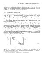
reached. Figure 3.29 displays
the
Laplaciari
pyramid
and its
frequency
resolution
for L = 3. It
shows that
x(n)
can
be
recovered perfectly
from
the
coarsest low-pass signal
x%(n)
and the
detail
signals,
d^n}^
di(ri),
and
do(n).
The
data
rate corresponding
to

each
of
these
signals
is
noted
on
this
figure. The net
rate
is the sum of
these
or
which
is
almost double
the
data
rate
in a
critically decimated
PR
dyadic tree.
This weakness
of the
Laplacian pyramid scheme
can be fixed
easily
if the
proper

antialiasing
and
interpolation
filters are
employed.
These
filters,
PR-QMFs,
also
provide
the
conditions
for the
decimation
and
interpolation
of the
high-frequency
signal
bands.
This
enhanced pyramid signal
representation
scheme
is
actually
identical
to the
dyadic
subbarid

tree, resulting
in
critical
sampling.
3.4.6
Modified
Laplacian Pyramid
for
Critical Sampling
The
oversampling
nature
of the
Laplacian pyramid
is
clearly undesirable, par-
ticularly
for
signal coding applications.
We
should also note
that
the
Laplaciari
pyramid does
not put any
constraints
on the
low-pass
antialiasing

and
interpola-
tion
filters,
although
it
decimates
the
signal
by 2.
This
is
also
a
questionable point
in
this approach.
In
this section
we
modify
the
Laplacian pyramid structure
to
achieve critical
sampling.
In
other words,
we
derive

the filter
conditions
to
decimate
the
Laplacian
error signal
by 2 and to
reconstruct
the
input signal perfectly.
Then
we
point
out
the
similarities between
the
modified
Laplacian pyramid
and
two-band
PR QMF
banks.
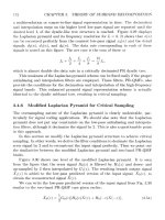
Figure 3.30 shows
one
level
of the
modified
Laplacian pyramid.

It is
seen
from
the figure
that
the
error signal
DQ(Z)
is filtered by
H\(z)
and
down-
and
up-sampled
by 2
then interpolated
by
G\(z}.
The
resulting branch output signal
X\(z]
is
added
to the
low-pass predicted version
of the
input signal,
XQ(Z],
to
obtain

the
reconstructed signal
X(z).
We
can
write
the
low-pass predicted version
of the
input signal
from
Fig. 3.30
similar
to the
two-band
PR-QMF
case given earlier,
3.4.
TWO-CHANNEL
FILTER BANKS
158
Figure
3.30:
Modified
Laplacian pyramid structure allowing
perfect
reconstruction
with
critical number
of

samples.
and the
Laplacian
or
prediction error signal
is
obtained.
As
stated
earlier
DQ(Z)
has the
full
resolution
of the
input signal
X(z).
Therefore
this structure oversamples
the
input signal. Now,
let us
decimate
and
interpolate this error signal. Prom Fig. 3.30,
If
we put
Eqs. (3.54)
and
(3.55)

in
this
equation,
and
then
add
XQ
and
X\,
we
get
the
reconstructed signal
154
CHAPTERS.
THEORY
OF
SUBBAND DECOMPOSITION
where
arid
If
we
choose
the
synthesis
or
interpolation
filters
as
the

aliasing terms cancel
and
as in Eq.
(3.37)
except
for the
inconsequential
z
1
factor.
One way of
achiev-
ing
PR is to let
HQ(Z),
H\(z]
be the
paraunitary
pair
of Eq.
(3.38),
H\(z)
=
z
-(
N
-i)
H
^_
z

-i^
and
then
golye
the
resu
}
ting
Eq
(3.40),
or Eq.
(3.47)
in the
time-domain.
This solution implies
that
all
filters,
analysis
and
synthesis, have
the
same length
N.
Furthermore,
for
h(n]
real,
the
magnitude responses

are
mirror
images,
implying equal bandwidth low-pass
and
high-pass
filters. In the
2-band
orthonor-
mal
PR-QMF case discussed
in
Section 3.5.4,
we
show
that
the
paraunitary solu-
tion
implies
the
time-domain orthonormality conditions
These equations
state
that
sequence
(/io(^)}
is
orthogonal
to its own

even trans-
lates
(except
n=0),
and
orthogonal
to
{hi(n}}
and its
even translates.
3,4.
TWO-CHANNEL FILTER BANKS
155
Vetterli
and
Herley (1992), proposed
the PR
biorthogonal
two-band
filter
bank
as an
alternative
to the
paraunitary solution. Their solution achieves zero aliasing
by
Eq.
(3.60).
The
PR

conditions
for
T(z)
is
obtained
by
satisfying
the
following
biorthogonal
conditions (Prob. 3.28):
where
These biorthogonal
niters
also provide basis sequences
in the
design
of
biorthogonal
wavelet
transforms discussed
in
Section 6.4.
The
low-
and
high-pass
filters
of a
two-

band
PR filter
bank
are not
mirrors
of
each other
in
this
approach.
Biorthogonality
provides
the
theoretical basis
for the
design
of PR filter
banks with linear-phase,
unequal bandwidth low-high
filter
pairs.
The
advantage
of
having linear-phase
filters in the PR filter
bank, however,
may
very
well

be
illusory
if we do not
monitor their
frequency
behavior.
As
mentioned earlier,
the filters in a
multirate structure should
try to
realize
the
antialiasing requirements
so as to
minimize
the
spillover
from
one
band
to
another.
This
suggests
that
the filters
HQ(Z]
and
H\(z]

should
be
equal bandwidth low-pass
and
high-pass respectively,
as in the
orthonormal solution.
This derivation shows
that
the
modified
Laplacian pyramid with critical sam-
pling
emerges
as a
biorthogonal two-band
filter
bank
or,
more desirably,
as
an
orthonormal two-band PR-QMF bank based
on the filters
used.
The
concept
of
the
modified Laplacian pyramid emphasizes

the
importance
of the
decimation
and
interpolation
filters
employed
in a
multirate signal processing structure.
3.4.7
Generalized
Subband
Tree Structure
The
spectral
analysis schemes considered
in the
previous sections assume
a
two-
band
frequency
split
as the
main decomposition operation.
If the
signal energy
is
concentrated mostly around

u
=
7r/2,
the
binary spectral split becomes
inefficient.
As
a
practical solution
for
this scenario,
the
original spectrum should
be
split into
three equal bands. Therefore
a
spectral division
by 3
should
be
possible.
The
three-band
PR, filter
bank
is a
special case
of the
M-band

PR filter
bank presented
in
Section 3.5.
The
general tree structure
is a
very practical
and
powerful
spectral
analysis technique.
An
arbitrary general
tree
structure
and its
frequency resolution
156
CHAPTER
3.
THEORY
OF
SUBBAND
DECOMPOSITION
are
displayed
in
Fig. 3.26
for L

=
3
with
the
assumption
of
ideal decimation
and
interpolation
filters.
The
irregular subband tree concept
is
very
useful
for
time-frequency
signal
analysis-synthesis purposes.
The
irregular tree structure should
be
custom
tai-
lored
for the
given input source. This suggests
that
an
adaptive tree structuring

algorithm
driven
by the
input signal
can be
employed.
A
simple tree structuring
algorithm
based
on the
energy compaction criterion
for the
given input
is
proposed
in
Akarisu
and Liu
(1991).
We
calculated
the
compaction gain
of the
Binomial
QMF
filter
bank (Section
3.6.1)

for
both
the
regular
and the
dyadic tree configurations.
The
test
results
for a
one-dimensional AR(1) source with
p —
0.95
are
displayed
in
Table
3.1
for
four-,
six-,
and
eight-tap
filter
structures.
The
term
Gj?
c
is the

upper bound
for
GTC
as
defined
in Eq.
(2.97)
using ideal
filters. The
table shows
that
the
dyadic
tree achieves
a
performance very close
to
that
of the
regular tree,
but
with
fewer
bands
and
hence reduced complexity.
Table
3.2
lists
the

energy compaction performance
of
several decomposition
techniques
for the
standard
test
images:
LENA,
BUILDING, CAMERAMAN,
and
BRAIN.
The
images
are of 256 x 256
pixels monochrome with
8
bits/pixel
resolution.
These
test
results
are
broadly consistent with
the
results obtained
for
AR(1) signal sources.
For
example,

the
six-tap
Binomial
QMF
outperformed
the
DOT
in
every case
for
both regular
and
dyadic tree configurations. Once again,
the
dyadic tree with
fewer
bands
is
comparable
in
performance
to the
regular
or
full
tree. However,
as
we
alluded
to

earlier, more levels
in a
tree tends
to
lead
to
poor band isolation.
This aliasing could degrade performance perceptibly under
low bit
rate
encoding.
3.5
M-Band
Filter
Banks
The
results
of the
previous two-band
filter
bank
are
extended
in two
directions
in
this
section. First,
we
pass

from
two-band
to
M-band,
and
second
we
obtain
more
general perfect reconstruction (PR) conditions
than
those
obtained
previously.
Our
approach
is to
represent
the filter
bank
by
three equivalent structures, each
of
which
is
useful
in
characterizing
particular
features

of the
subband system.
The
conditions
for
alias
cancellation
and
perfect reconstruction
can
then
be
described
in
both time
and
frequency domains using
the
polyphase decomposition
and the
alias
component (AC)
matrix
formats.
In
this
section,
we
draw heavily
on the

papers
by
Vaidyanathan (ASSP
Mag.,
1987),
Vetterli
and
LeGall (1989),
and
Malvar
(Elect.
Letts.,
1990)
and
attempt
to
establish
the
commonality
of
these
3.5,
M-BAND
FILTER
BANKS
(a)
4-tap
Binomial-QMF.
level
1

2
3
4
Regular Tree
#
of
bands
2
4
8
16
GTC
3.6389
6.4321
8.0147
8.6503
Gfr
3.9462
7.2290
9.1604
9.9407
Half
Band
lire
gular Tree
#
of
bands
2
3

4
5
GTC
3.63S9
6.3681
7.8216
8.3419
GTC
3.9462
7.1532
8.9617
9,6232
(b)
6-tap Binomial-QMF.
level
1
2
3
4
Regular Tree
#
of
bands
2
4
8
16
GTC
3.7608
6.7664

8.5291
9.2505
GTC
3.9462
7.2290
9.1604
9.9407
Half
Band
Irre
gular
Tree
#
of
bands
2
3
4
5
GTC
3.7608
6.6956
8.2841
8.8592
GTC
3.9462
7,1532
8.9617
9.6232
(c)

8-tap
Binomial-QMF.
level
1
2
3
4
Regular
Tree
#
of
bands
2
4
8
16
Grc
3.8132
6.9075
8.7431
9.4979
{*fQ
3.9462
7.2290
9.1604
9.9407
Half
Band Irre gular Tree
#
of

bands
2
3
4
5
GTC
3.8132
6.8355
8.4828
9.0826
GTC
3.9462
7.1532
8.9617
9.6232
Table
3.1:
Energy
compaction
performance
of
PR-QMF
filter
banks
along
with
the
full
tree
and

upper
performance
bounds
for
AR(1)
source
of p
—
0.95.
TEST
IMAGE
8
x 8 2D DCT
64
Band Regular 4-tap
B-QMF
64
Band Regular
6-tap
B-QMF
64
Band Regular
8-tap
B-QMF
4
x 4 2D DCT
16
Band Regular
4-tap
B-QMF

16
Band Regular
6-tap
B-QMF
16
Band Regular
8-tap
B-QMF
*10
Band Irregular
4-tap
B-QMF
"10
Band Irregular
6-tap
B-QMF
*10
Band Irregular 8-tap B-QMF
LENA
21.99
19,38
22.12
24.03
16.00
16.TO
18.99
20.37
16.50
18.65
19.66

BUILDING
20.08
18.82
21.09
22.71
14.11
15.37
16.94
18.17
14.95
16.55
17.17
CAMERAMAN
19.10
18.43
20.34
21.45
14.23
15.45
16.91
17.98
13.30
14.88
15.50
BRAIN
3.79
3.73
3.82
3.93
3.29

3.25
3.32
3.42
3 .34
3 .66
3
.75
Bands
used
are
//////
-
Ulllh
~
llllhl
-
llllhh
-
lllh
-
llhl
-
Uhh
~lh-kl-
hh.
Table
3.2:
Compaction
gain,
GTC,

°f
several
different
regular
and
dyadic
tree
structures
along
with
the DCT for the
test
images.
158
CHAPTER
3.
THEORY
OF
SUBBAND
DECOMPOSITION
approaches,
which
in
turn reveals
the
connection
between
block
transforms,
lapped

transforms,
and
subbands.
3,5.1
The
M-Band
Filter Bank Structure
The
M-band
QMF
structure
is
shown
in
Fig. 3.31.
The
bank
of filters
{Hk(z),
k —
0,1, ,
M
—
1}
constitute
the
analysis
filters
typically
at the

transmitter
in a
signal
transmission
system. Each
filter
output
is
subsampled,
quantized
(i.e.,
coded),
and
transmitted
to the
receiver,
where
the
bank
of
up-samplers/synthesis
filters
reconstruct
the
signal.
In
the
most general case,
the
decimation

factor
L
satisfies
L
<
M and the
filters
could
be any mix of
FIR
and
IIR
varieties.
For
most practical cases,
we
would
choose maximal decimation
or
"critical subsampling,"
L =
M.
This
ensures
that
the
total
data
rate
in

samples
per
second
is
unaltered
from
x(ri)
to the set of
subsampled
signals,
{^jt(n),
k
=
0,1, ,
M
—
1}.
Furthermore,
we
will
consider
FIR
filters of
length
N at the
analysis side,
and
length
N for the
synthesis

filters.
Also,
for
deriving
PR
requirements,
we do not
consider coding errors. Under
these
conditions,
the
maximally decimated M-band
FIR QMF filter
bank structure
has
the
form
shown explicitly
in
Fig. 3.32. [The term
QMF
is a
carryover
from
the
two-band
case
and has
been used, somewhat loosely,
in the DSP

community
for
the
M-band case
as
well.l
Figure
3.31:
M-band
filter
bank.
3.5.
M-BAND
FILTER BANKS
159
Figure
3.32: Maximally decimated
M-band
FIR QMF
structures.
Prom this block diagram,
we can
derive
the
transmission features
of
this
sub-
band system.
If we

were
to
remove
the up- and
down-samplers
from
Fig. 3.32,
we
would
have
and
perfect reconstruction; i.e.,
y(n)
—
x(n
— no) can be
realized with relative
ease,
but
with
an
attendant
M-fold
increase
in the
data
rate.
The
requirement
is

obviously
and
i.e.,
the
composite transmission reduces
to a
simple delay.
Now
with
the
samplers reintroduced,
we
have,
at the
analysis side.
at the
synthesis side.
The
sampling bank
is
represented using Eqs. (3.12)
and
(3.9)
in
Section 3.1.1,
160
CHAPTER
3.
THEORY
OF

SUBBAND
DECOMPOSITION
where
W
—
e~~
j27r
/
M
.
Combining these
gives
We
can
write this
last
equation more compactly
as
where
HAC(Z]
is the
a/ms
component,
or
^4C
matrix.
The
subband
filter
bank

of
Fig. 3.32
is
linear,
but
time-varying,
as can be
inferred
from
the
presence
of the
samplers. This
last
equation
can be
expanded
as
Three kinds
of
errors
or
undesirable distortion terms
can be
deduced
from
this
last
equation.
(1)

Aliasing
error
or
distortion
(ALD) terms. More properly,
the
subsam-
pling
is the
cause
of
aliasing components while
the
up-samplers
produce images.
3.5.
M-BAND
FILTER BANKS
161
The
combination
of
these
is
still called aliasing. These aliasing terms
in Eq.
(3.73)
can
be
eliminated

if we
impose
In
this
case,
the
input-output
relation
reduces
to
just
the first
term
in Eq.
(3.73),
which
represents
the
transfer
function
of a
linear, time-invariant system:
(2)
Amplitude
and
Phase
Distortion.
Having constrained
{Hk,Gk}
to

force
the
aliasing term
to
zero,
we are
left
with classical magnitude (amplitude)
arid
phase distortion, with
Perfect
reconstruction requires T(z)
= z
n
°,
a
pure delay,
or
Deviation
of
\T(e^}\
from
unity constitutes amplitude distortion,
and
deviation
of
(f)(uj)
from
linearity
is

phase distortion. Classically,
we
could select
an
IIR
all-
pass
filter
to
eliminate magnitude distortion, whereas
a
linear-phase FIR, easily
removes
phase
distortion.
When
all
three distortion terms
are
zero,
we
have
perfect
reconstruction:
The
conditions
for
zero aliasing,
and the
more stringent

PR, can be
developed
using
the AC
matrix formulation,
and as we
shall see,
the
polyphase decomposition
that
we
consider next.
3.5.2
The
Polyphase
Decomposition
In
this
subsection,
we
formulate
the PR
conditions
from
a
polyphase
representation
of
the
filter

bank. Recall
that
from
Eqs. (3.14)
and
(3.15), each analysis
filter
H
r
(z]
can be
represented
by
162
CHAPTER
3.
THEORY
OF
SUBBAND DECOMPOSITION
Figure 3.33: Polyphase decomposition
of
H
r
(z).
These
are
shown
in
Fig. 3.33.
When this

is
repeated
for
each analysis
filter, we can
stack
the
results
to
obtain
where
'Hp(z)
is the
polyphase matrix,
and
Z_
M
is a
vector
of
delays
and
Similarly,
we can
represent
the
synthesis
filters
by
3.5.

M-BAND
FILTER
BANKS
163
This
structure
is
shown
in
Fig. 3.34.
Figure
3.34: Synthesis
filter
decomposition.
In
terms
of the
polyphase components,
the
output
is
The
reason
for
rearranging
the
dummy indexing
in
these
last

two
equations
is to
obtain
a
synthesis polyphase representation with delay arrows pointing down,
as
164
CHAPTER
3.
THEORY
OF
SUBBAND
DECOMPOSITION
in
Fig.
3.34(b).
This last equation
can now be
written
as
where
The
synthesis polyphase matrix
in
this last equation
has a
row-column
indexing
different from

H
p
(z)
in Eq.
(3.81).
For
consistency
in
notation,
we
introduce
the
"counter-identity"
or
interchange
matrix
J,
with
the
property
that
pre(post)multiplication
of a
matrix
A by J
interchanges
the
rows (columns)
of
vl,

i.e.,
Also
note
that
and
We
have already employed this notation, though somewhat implicitly,
in the
vector
of
delays:
3.5.
M-BAND
FILTER BANKS
165
With
this convention,
and
with
Q
p
(z)
defined
in the
same
way as
l~ip(z]
of
Eq.
(3.81),

i.e.,
by
we
recognize
that
the
synthesis polyphase matrix
in Eq.
(3.86)
is
This permits
us to
write
the
polyphase synthesis equation
as
Note
that
we
have
defined
the
analysis
and
synthesis polyphase matrices
in
exactly
the
same
way so as to

result
in
Figure
3.35: Polyphase representation
of QMF filter
bank.
Finally,
we see
that
Eqs. (3.81)
and
(3.94)
suggest
the
polyphase block diagram
of
Fig. 3.35.
As
explained
in
Section 3.1.2,
we can
shift
the
down-samplers
to the
left
of the
analysis polyphase matrix
and

replace
Z
M
by z in the
argument
of
166
CHAPTER
3.
THEORY
OF
SUBBAND
DECOMPOSITION
Figure
3.36: Equivalent polyphase
QMF
bank.
7i
p
(.).
Similarly,
we
shift
the
up-samplers
to the
right
of the
synthesis polyphase
matrix

and
obtain
the
structure
of
Fig. 3.36. These
two
polyphase structures
are
equivalent
to the filter
bank with which
we
started
in
Fig. 3.32.
We
can
obtain still another representation, this time with
the
delay arrows
pointing
up, by the
following
manipulations. From
Eq.
(3.81), noting
that
J
2

=
I,
we
can
write
Similarly,
These
last
two
equations
define
the
alternate polyphase
QMF
representations
of
Figs.
3.37
and
3.38,
where
we are
using
It is now
easy
to
show
that
(Prob. 3.14)
3.5.

M-BAND
FILTER
BANKS
16'
Figure
3.37: Alternative polyphase structure.
Figure 3.38: Alternative polyphase representation.
Either
of the
polyphase representations allow
us to
formulate
the PR
require-
ments
in
terms
of the
polyphase matrices. Prom Fig. 3.36.
we
have
which
defines
the
composite structure
of
Fig. 3.39.
The
condition
for PR in Eq.

(3.78)
was
T(z]
=
z~~
n
°.
It is
shown
by
Vaidya-
nathan
(April
1987)
that
PR is
satisfied
if
where
I
m
denotes
the
mxm
identity matrix.
This
condition
is
very broadly
stated.

Detailed discussion
of
various special cases induced
by
imposing symmetries
on
168
CHAPTER
3.
THEORY
OF
SUBBAND
DECOMPOSITION
Figure
3.39: Composite
M-band
polyphase structure.
the
analysis-synthesis
filters can be
found
in
Viscito
and
Allebach
(1989).
For our
purposes
we
will

only consider
a
sufficient
condition
for PR,
namely,
(This corresponds
to the
case where
&o
— 0.) For if
this
condition
is
satisfied,
using
the
manipulations
of
Fig. 3.40,
we can
demonstrate
that
(Prob. 3.13)
The
bank
of
delays
is
moved

to the
right
of the
up-samplers,
and
then out-
side
of the
declinator-interpolator
structure.
It is
easily
verified
that
the
signal
transmission
from
point
(1) to
point
(2) in
Fig.
3.40(c)
is
just
a
delay
of M —
I

units.
Thus
the
total transmission
from
x(n)
to
y(n)
is
just
[(M
—
1)
-f
Mfj,\
delays,
resulting
in
T(z]
=
z~
n
°.
Thus
we
have
two
representations
for the
M-band

filter
bank,
the AC
matrix
approach,
and the
polyphase decomposition.
We
next develop detailed
PR
filter
bank requirements using each
of
these
as
starting
points.
The AC
matrix provides
a
frequency-domain formulation, while
the
polyphase
is
useful
for
both
frequency-
and
time-domain interpretations.

We
close
this
subsection
by
noting
the
relation-
ship between
the AC and
polyphase matrices. From
Eq.
(3.72),
we
know
that
the
AC
matrix
is
1=0
Substituting
the
polyphase expansion
from
Eq.
(3.79) into this
last
equation
gives

',5.
M-BAND
FILTER BANKS
169
Figure 3.40: Polyphase implementation
of PR
condition
of Eq.
(3.100).
This
last
equation
can be
expressed
as the
product
of
three matrices,
170
CHAPTER
3.
THEORY
OF
SUBBAND DECOMPOSITION
where
W
is the DFT
matrix,
and
A(z]

is the
diagonal matrix
We
can
now
develop
filter
bank properties
in
terms
of
either
HAC(
Z
]
°
r
%p(
z
)
or
both.
3.5.3
PR
Requirements
for FIR
Filter
Banks
A
simplistic approach

to
satisfying
the PR
condition
in Eq.
(3.100)
is to
choose
Q'
p
(z)
=
z~^7ip
l
(z).
Generally this implies that
the
synthesis
filters
would
be
IIR
and
possibly unstable, even when
the
analysis
filters are
FIR. Therefore,
we
want

to
impose conditions
on the FIR
H.
p
(z)
that
result
in
synthesis
filters
which
are
also FIR. Three conditions
are
considered (Vetterli
and
LeGall,
1989).
(1)
Choose
the FIR
H
P
(z}
such
that
its
determinant
is a

pure
delay
(i.e.,
dei{H
p
(z]}
is a
monomial),
where
p is an
integer
>
0.
Then
we can
satisfy
Eq.
(3.100) with
an FIR
synthesis
bank.
The
sufficiency
is
established
as
follows.
We
want
Multiply

by
H
p
l
(z)
and
obtain
The
elements
in the
adjoint matrix
are
just cofactors
of
"H
p
(z),
which
are
products
and
sums
of FIR
polynomials
and
thus
FIR. Hence, each element
of
O
p

(z)
is
equal
to the
transposed
FIR
cofactor
of
H
p
(z)(within
a
delay).
This
approach
generally
leads
to FIR
synthesis
filters
that
are
considerably longer
than
the
analysis
filters.
(2)
The
second class

consists
of PR filters
with equal length
analysis
and
syn-
thesis
filters.
Conditions
for
this using
a
time-domain formulation
are
developed
in
Section 3.5.5.
(3)
Choose
'Hp(z)
to be
paraunitary
or
"lossless." This results
in
identical
analysis
and
synthesis
filters

(within
a
time-reversal),
which
is the
most commonly
3.5.
M-BAND
FILTER
BANKS
171
stated condition.
A
lossless
or
paraunitary
matrix
is
defined
by the
property
The
delay
no is
selected
to
make
G
p
(z)

the
polyphase matrix
of a
causal
filter
bank.
The
converse
of
this theorem
is
also valid.
We
will
return
to
review
cases
(1) and (2)
from
a
time-domain standpoint.
Much
of the
literature
on PR
structures deals with paraunitary solutions
to
which
we

now
turn.
3.5.4
The
Paraunitary
FIR
Filter Bank
We
have shown
that
PR is
assured
if the
analysis polyphase matrix
is
lossless
(which
also
forces
losslessness
on the
synthesis
matrix).
The
main
result
is
that
the
impulse

responses
of the
paraunitary
filter
bank must
satisfy
a set of
orthonormal
constraints,
which
are
generalizations
of the M — 2
case dealt with
in
Section 3.4.
(See
also Prob. 3.17)
First,
we
note
that
the
choice
of
G
p
(z)
in Eq.
(3.109) implies

that
each synthesis
filter
is
just
a
time-reversed version
of the
analysis
filter,
And,
if
this condition
is
met,
we can
simply choose
This results
in
To
prove this, recall
that
the
polyphase decomposition
of the filter
bank
is
But,
from
Eq.

(3.109),
we had
or
172
CHAPTER
3.
THEORY
OF
SUBBAND DECOMPOSITION
Now
let's replace
z by
Z
M
,
and
multiply
by
JZ_M
t
|Q
obtain
=
z~
T
h(z-
1
),
(3.112)
where

r =
[Mn
0
+
(M-l)].
Thus
G^(z)
=
z~
r
H
k
(z),
k -
0,1, ,
M-1
as
asserted
in
Eq.
(3.110).
We
can
also write
the
paraunitary
PR
conditions
in
terms

of
elements
of the
AC
matrix.
In
fact,
we can
show
that
lossless
T~i
p
(z)
implies
a
lossless
AC
matrix
arid
conversely,
that
is,
where
and the
subscripted asterisk implies conjugation
of
coefficients
in the
matrix.

The
proof
is
straightforward. Prom
Eq.
(3.104)
But
for a
DFT
matrix. Hence
f~Tt
. 1 .
The AC
matrix approach
will
allow
us to
obtain
the
properties
of filters in
lossless structures. Prom
Eq.
(3.72),
we had
where
HAC(Z)
is the AC
matrix.
For

zero aliasing,
we had in Eq.
(3.74)
3.5.
M-BAND
FILTER BANKS
173
Let
us
substitute successively
zW,
zW
2
, ,
zW
M
~
l
for z in
this last equation.
Each substitution
of zW in the
previous equation induces
a
circular
shift
in the
rows
of
HAC-

For
example,
can be
rearranged
as
This permits
us to
express
the set of M
equations
as one
matrix equation
of the
form
where
G\
c
(z]
is the
transpose
of the AC
matrix
for the
synthesis
filters.
Equation (3.114) constitutes
the
requirements
on the
analysis

and
synthesis
AC
matrices
for
alias-free
signal reconstructions
in the
broadest possible terms.
If
we
impose
the
additional constraint
of
perfect
reconstruction,
the
requirement
becomes
The PR
requirements
can be met by
choosing
the AC
matrix
to be
lossless.
The
imposition

of
this requirement
will
allow
us to
derive time-
and
frequency-domain
properties
for the
paraunitary
filter
bank. Thus,
we
want
174
CHAPTER
3.
THEORY
OF
SUBBAND
DECOMPOSITION
We
will
show
that
the
necessary
and
sufficient

conditions
on filter
banks sat-
isfying
the
paraunitary
condition
are
as
follows.
Let
Then
We
will
first
interpret these results,
and
then provide
a
derivation.
For
r
=
5,
we see
that
p
rr
(Mn)
=

S(n}.
Hence
&
rr
(z]
—
H
r
(z~
1
}H
r
(z)
is the
transfer
function
of an
M
th
band
filter, Eq.
(3.25),
and
H
r
(z)
must
be a
spectral
factor

of
<&
rr
(z).
In the
time-domain,
the
condition
is
which
implies
that
the
impulse response
h
r
(n}:
The
latter asserts
that
{h
r
(k}}
is
orthogonal
to its
translates
shifted
by
M.

For
r
=£
s, we
have
p
rs
(Mn)
— 0, or
This implies
{h
r
(k}}
is
orthogonal
to
{h
s
(k}}
and to all M
translates
of
{h
s
(k)}
This
condition corresponds
to the
off-diagonal
terms

in Eq.
(3.116).
It
is a
time-
domain equivalent
of
aliasing cancellation.
The
paraunitary requirement therefore imposes
a set of
orthonormality
re-
quirements
on the
impulse responses
in the
analysis
filter
bank
and by Eq.
(3.112)
on
the
synthesis
filters as
well.
Another version
of
this

will
be
developed
in
Section
3.5.5
in
conjunction with
the
polyphase matrix approach.
3.5.
M-BAND
FILTER BANKS
175
Another
consequence
of a
paraunitary
AC
matrix
is
that
the filter
bank
is
power
complementary,
which
means
that

To
appreciate this, note
that
if
HAC(
Z
]
i
g
lossless, then
H^
c
(z}
is
also lossless.
Then
H^
C
(Z)HAC(
Z
)
—
MI,
and the first
diagonal element
is
just
Now
for the
proof

of Eq.
(3.118): First
we
define
The
following
are
Fourier transform pairs:
The
condition
to be
satisfied,
Eq,
(3.116),
is
In
the
time-domain, this becomes
But
176
CHAPTERS.
THEORY
OF
SUBBAND
DECOMPOSITION
Equation (3.124) becomes
The
product
of
this sampling

function
with
p
rs
(n)
leaves
us
with
p
rs
(Mri]
on the
left-hand
side
of Eq.
(3.126)
which completes
the
proof.
On
occasion, necessary conditions
for a
paraunitary
filter
bank
are
confused
with
sufficient
conditions.

Our
solution,
Eq.
(3.118), implies
a
paraunitary
filter
bank.
The
M
th
band
filter
requirement,
Eq.
(3.119),
and the
power comple-
mentary property
of Eq.
(3.122)
are
consequences
of the
paraunitary
filter
bank.
Together they
do
not

imply
Eq.
(3.116).
The
additional requirement
of Eq.
(3.121)
must also
be
observed.
One
can
start
with
a
prototype low-pass
HQ(Z),
satisfying
the
M
th
band
re-
quirement
HO(Z)HQ(Z~
I
)
—
&QQ(Z)
and

develop
a
bank
of filters
from
This selection satisfies power complementarity
and
M
th
band
requirement,
but
is
not
necessarily paraunitary.
Another
difficulty
with this
M
th
band design
is
evident
in
this
last
equation.
First,
H
r

(z)
can
have complex
coefficients
resulting
in
complex
subband
signals.
Secondly,
as
Vaidyanathan
(April
1987) points out,
the
aliasing cancellation
re-
quired
by Eq.
(3.116)
for r
^
s is
difficult
to
realize when
HQ(Z)
is a
sharp low-
pass

filter. It
turns
out
that
alias
cancellation
and
sharp
cutoff
filters are
largely
incompatible
in
this
design.
For
this reason
we
turn
to
alternate product-type
realizations
of
lossless
filter
banks.
The
Two-Band
Case
To

fix
ideas,
we
particularize these results
for the
case
M = 2 and
demonstrate
the
consistency with
the
two-band paraunitary
filter
bank derived
in
Section 3.3.
For
alias cancellation
from
Eq.
(3.114),
we
want (real
coefficients
are
assumed
The sum in
this
last
equation

is
recognized
as the
sampling
function
of Eq.
(3.4)