Multiresolution Signal Decomposition Transforms, Subbands, and Wavelets phần 2 potx
Bạn đang xem bản rút gọn của tài liệu. Xem và tải ngay bản đầy đủ của tài liệu tại đây (2.54 MB, 54 trang )
34
CHAPTER
2.
ORTHOGONAL TRANSFORMS
For
completely decorrelated spectral
coefficients,
rj
c
=
I.
The
second parameter
TJE
measures
the
energy compaction property
of the
transform.
Defining
J'
L
as the
expected value
of the
summed squared error
J/,
of
Eq.
(2.20)
This
J'
L
has
also been called
the
basis
restriction,
error
by
Jain
(1989). Then
the
compaction
efficiency
is
Thus
rjpj
is the
fraction
of the
total
energy
in the first L
components
of
0,
where
{0f}
are
indexed according
to
decreasing value.
The
unitary transformation
that
makes
r\
c
= 0 and
minimizes
J'
L
is the
Karhu-
nen-Loeve
transform (Karhunen, 1947;
Hotellirig,
1933).
Our
derivation
for
real
signals
and
transforms
follows.
Consider
a
unitary transformation
$
such
that
The
approximation
/,
and
approximation error
e
L
are
By
orthonormality,
it
easily
follows
that
2.2.
TRANSFORM EFFICIENCY
AND
CODING PERFORMANCE
35
From
Eq.
(2.34),
Therefore,
so
that
the
error measure becomes
To
obtain
the
optimum transform,
we
want
to find the
$
r
that
minimizes
J'
L
for
a
given
L,
subject
to the
orthonormality
constraint,
^^_
s
—
6
r
-s-
Using
Lagrangian
multipliers,
we
minimize
Each
term,
in the sum is of the
form
Taking
the
gradient
4
of
this with respect
to
x
(Prob. 2.6),
or
Doing
this
for
each term
in Eq.
(2.74)
gives
which
implies
where
4
The
gradient
is a
vector
defined
as
36
CHAPTER
2.
ORTHOGONAL TRANSFORMS
(The
reason
for the
transpose
is
that
we had
defined
$
r
as the
rth
column
of
$.)
Hence
3>
r
is an
eigenvector
of the
signal covariance matrix
Rf,
and
A
r
,
the
associated eigenvalue,
is a
root
of the
characteristic polynomial,
det(\I
—
R/).
Since
Rf is a
real, symmetric matrix,
all
{A;}
are
real, distinct,
arid
nonnegative.
The
value
of the
minimized
J'
L
is
then
The
covariance matrix
for the
spectral
coefficient
vector
is
diagonal,
as can be
seen
from
Thus
4>
is the
unitary matrix
that
does
the
following:
(1)
generates
a
diagonal
RQ
and
thus completely decorrelates
the
spectral
coeffi-
cients resulting
in
r?
c
— 1,
(2)
repacks
the
total
signal energy among
the first
L
coefficients,
maximizing
TJE*
It
should
be
noted,
however,
that
while many
matrices
can
decorrelate
the
input signal,
the KLT
both decorrelates
the
input
perfectly
and
optimizes
the
repacking
of
signal energy. Furthermore,
it is
unique.
The
difficulty
with
this
transformation
is
that
it is
input signal
specific—i.e.,
the
matrix
$
T
consists
of the
eigenvectors
of the
input covariance matrix
Rf.
It
does provide
a
theoretical limit
against which signal-independent transforms (DFT,
DOT,
etc.)
can be
compared.
In
fact,
it is
well
known
that
for an
AR(1) signal source
Eq.
(2.61)
with
p
large,
on
the
order
of
0.9,
the DCT
performance
is
very close
to
that
of the
KLT.
A
frequently
quoted result
for the
AR(1) signal
and N
even (Ray
and
Driver. 1970)
is
where
{&k}
are the
positive
roots
of
This
result
simply underscores
the
difficulty
in
computing
the KLT
even when
applied
to the
simplest, nontrivial signal model.
In the
next section,
we
describe
other
fixed
transforms
and
compare them with
the
KLT. (See also Prob. 2.19)
2.2,
TRANSFORM EFFICIENCY
AND
CODING PERFORMANCE
37
For
p
=
0.91
in the
AR(1) model
and N - 8,
Clarke (1985)
has
calculated
the
packing
and
decorrelation
efficiencies
of the KLT and the
DCT:
f\E
WE
L
KLT
DCT
1
79.5
79.3
2
91.1
90.9
3
94.8
94.8
4
96.7
96.7
5
97.9
97.9
6
98.7
98.7
7
99.4
99.4
8
100
100
These numbers speak
for
themselves. Also
for
this example,
t]
c
=
0.985
for the
DCT
compared with
1.0 for the
KLT.
2.2.2
Comparative
Performance
Measures
The
efficiency
measures
r\
c
,
TIE
in
Section 2.2.1 provide
the
bases
for
comparing
unitary transforms against each other.
We
need, however,
a
performance measure
that
ranges
not
only over
the
class
of
transforms,
but
also over
different
coding
techniques.
The
measure introduced here serves
that
purpose.
In all
coding techniques, whether they
be
pulse code modulation (PCM),
differ-
ential pulse code modulation
(DPCM),
transform coding
(TC),
or
subband coding
(SBC),
the
basic performance measure
is the
reconstruction error
(or
distortion)
at a
specified information
bit
rate
for
storage
or
transmission.
We
take
as the
basis
for all
comparisons,
the
simplest coding scheme, namely
the
PCM,
and
compare
all
others
to it.
With respect
to
Fig. 2.3,
we see
that
PCM
can be
regarded
as a
special case
of TC
wherein
the
transformation matrix
<3>
is
the
identity matrix
I, in
which case
we
have simply
0_
—
f.
The
reconstruction
error
is
/
as
defined
by Eq.
(2.38),
and the
mean square reconstruction error
is
of
The TC
performance measure compares
of for TC to
that
for
PCM. This
measure
is
called
the
gain
of
transform coding over
PCM and
defined
(Jayant
and
Noll,
1984)
as
In the
next chapter
on
subband
coding,
we
will
similarly
define
38
CHAPTER
2.
ORTHOGONAL TRANSFORMS
In
Eq,
(2.39)
we
asserted that
for a
unitary transform,
the
mean
square
le
construction
error equals
the
mean square quantization error.
The
pioof
is
eas\
Since
then
~T
where
#
is the
quantization error vector.
The
average mean square
(m.s.)
error
(or
distortion)
is
where
<j'
2
a
is the
variance
of the
quantization
error
in the
K
ih
spectral
coefficient.
as
depicted
in
Fig. 2.6.
Suppose
that
Rk
bits
are
allocated
to
quantizer
Q^.
Then
we can
choose
the
quantizer
to
minimize
<r|
for
this value
of
R^
and the
given probability density
function
for
0^.
This
minimum mean square error quantizer
is
called
the
Lloyd-
Max
quantizer, (Lloyd, 1957; Max, 1960).
It
minimizes separately each
cr|
fc
,
and
hence
the sum
Y^k
a
q
k
-
The
structure
of
Fig.
2.6
suggests
that
the
quantizer
can
be
thought
of an
estimator, particularly
so
since
a
mean square error
is
being
minimized.
For the
optimal quantizer
it can be
shown
that
the
quantization error
is
unbiased,
and
that
the
error
is
orthogonal
to the
quantizer
output
(just
as in
the
case
for
optimal linear estimator), (Prob. 2.9)
Figure 2.6:
The
coefficient
quantization error.
2.2.
TRANSFORM EFFICIENCY
AND
CODING PERFORMANCE
39
The
resulting mean square error
or
distortion, depends
on the
spectral
coeffi-
cient
variance
er|.,
the
pdf,
the
quantizer
(in
this case.
Lloyd-Max),
and the
number
of
bits
Rk
allocated
to the
kth
coefficient.
From rate-distortion
theory
(Berger.
1971),
the
error
variance
can be
expressed
as
where
f(Rk)
is the
quantizer
distortion
function
for a
unity variance input. Typ-
ical
I
v.
where
7^
depends
on the pdf for
Ok
and on the
specific
quantizer. Jayant
and
Noll
(1984) report values
of 7 =
1.0, 2.7, 4.5,
and 5.7 for
uniform,
Gaussian, Laplacian,
and
Gamma
pdfs,
respectively.
The
average mean square reconstruction error
is
then
Next,
there
is the
question
of bit
allocation
to
each
coefficient,
constrained
by
NR,
the
total number
of
bits available
to
encode
the
coefficient
vector
0
and R is the
average number
of
bits
per
coefficient.
To
minimize
Eq.
(2.89) subject
to the
constraint
of Eq.
(2.90),
we
again
resort
to
Lagrangian multipliers.
First
we
assume
7^
to be the
same
for
each
coefficient,
and
then solve
to
obtain (Prob. 2.7)
This result
is due to
Huang
and
Schultheiss (1963)
and
Segall (1976).
The
number
of
bits
is
proportional
to the
logarithm
of the
coefficient
variance,
or to the
power
in
that
band,
an
intuitively
expected
result.
40
CHAPTER
2.
ORTHOGONAL TRANSFORMS
It can
also
be
shown
that
the bit
allocation
of Eq.
(2.92)
results
in
equal
quantization error
for
each
coefficient,
and
thus
the
distortion
is
spread
out
evenly
among
all the
coefficients,
(Prob.
2.8)
The
latter also equals
the
average distortion, since
The
preceding result
is the pdf and
Rk
optimized distortion
for any
unitary
transform.
For the PCM
case,
$
=
/, and
of
reduces
to
There
is a
tacit
assumption here
that
the 7 in the PCM
case
of Eq,
(2.95)
is
the
same
as
that
for TC in Eq.
(2.93). This
may not be the
case when,
for
example,
the
transformation changes
the pdf of the
input signal.
We
will
neglect
this
effect.
Recall
from
Eq.
(2.63)
that,
for a
unitary transform,
The
ratio
of
distortions
in
Eqs.
(2.95)
and
(2.93)
gives
The
maximized
GTC is the
ratio
of the
arithmetic mean
of the
coefficient
variances
to the
geometric mean.
Among
all
unitary matrices,
the KLT
minimizes
the
geometric mean
of the
coefficient
variances.
To
appreciate this, recall
that
from
Eq.
(2.77)
the KLT
produced
a
diagonal
RQ,
so
that
2.3.
FIXED
TRANSFORMS
41
The
limiting value
of
GKLT
for IV
-^
oo
gives
an
upper bound
on
transform
coding
performance.
The
denominator
in Eq.
(2.99)
can be
expressed
as
Jayant
and
Noll (1984) show
that
where
Sf is the
power spectral density
of the
signal
Hence,
and the
numerator
in Eq.
(2.99)
is
recognized
as
Hence,
is
the
reciprocal
of the
spectral
flatness
'measure
introduced
by
Makhoul
and
Wolf
(1972).
It is a
measure
of the
predictability
of a
signal.
For
white noise,
°°GTC
— 1 and
there
is no
coding gain.
This
measure increases with
the
degree
of
correlation
and
hence predictability. Accordingly, coding gain increases
as the
redundancy
in the
signal
is
removed
by the
unitary transformation.
2.3
Fixed
Transforms
The KLT
described
in
Section
2.2 is the
optimal unitary transform
for
signal
cod-
ing
purposes.
But the
DOT
is a
strong competitor
to the KLT for
highly correlated
42
CHAPTER
2.
ORTHOGONAL
TRANSFORMS
signal sources.
The
important
practical
features
of the DCT are
that
it is
signal
independent (that
is, a fixed
transform),
and
there exist
fast
computational
al-
gorithms
for the
calculation
of the
spectral
coefficient
vector.
In
this section
we
define,
list,
and
describe
the
salient features
of the
most popular
fixed
transforms,
These
are
grouped into three categories: sinusoidal, polynomial,
and
rectangular
transforms.
2.3.1
Sinusoidal
Transforms
The
discrete Fourier transform (DFT)
and its
linear derivatives
the
discrete cosine
transform
(DCT)
and the
discrete sine transform (DST)
are the
main members
of
the
class described here.
2.3.1.1
The
Discrete
Fourier
Transform
The DFT is the
most important orthogonal transformation
in
signal analysis with
vast implication
in
every
field of
signal processing.
The
fast
Fourier transform
(FFT)
is a
fast
algorithm
for the
evaluation
of the
DFT.
The set of
orthogonal (but
not
normalized) complex sinusoids
is the
family
with
the
property
Most authors
define
the
forward
and
inverse
DFTs
as
The
corresponding matrices
are
This definition
is
consistent with
the
interpretation
that
the DFT is the
Z-trans-
from
of
{x(n}}
evaluated
at N
equally-spaced points
on the
unit circle.
The set
2.3.
FIXED
TRANSFORMS
43
of
coefficients
{X(k)}
constitutes
the
frequency
spectrum
of the
samples.
From
Eqs. (2.107)
and
(2.108)
we see
that
both
X(k)
and
x(n)
are
periodic
in
their
arguments with period
N.
Hence
Eq.
(2.108)
is
recognized
as the
discrete
Fourier
series
expansion
of the
periodic sequence
{:r(n)},
and
{X(k}}
are
just
the
discrete
Fourier series
coefficients
scaled
by
N.
Conventional
frequency
domain interpre-
tation permits
an
identification
of
X(0)/N
as the
"DC" value
of the
signal.
The
fundamental
(x'i(n)
=
e?
27rn
/
Ar
}
is a
unit vector
in the
complex plane
that
rotates
with
the
time index
n. The first
harmonic
{x%(ri)}
rotates
at
twice
the
rate
of
fundamental
and so on for the
higher harmonics.
The
properties
of
this transform
are
summarized
in
Table
2.1.
For
more details,
the
reader
can
consult
the
wealth
of
literature
on
this subject, e.g., Papoulis (1991),
Opperiheim
and
Schafer
(1975),
Haddad
and
Parsons
(1991).
The
unitary
DFT is
simply
a
normalized
DFT
wherein
the
scale factor
N
appearing
in
Eqs.
(2.106)-(2.109)
is
reapportioned
according
to
This makes
arid
the
unitary transformation matrix
is
From
a
coding
standpoint,
a key
property
of
this
transformation
is
that
the
basis vectors
of the
unitary
DFT
(the columns
of
$*)
are the
eigenvectors
of a
circulant
matrix.
That
is,
with
the
&
th
column
of
4>*
denoted
by
we
will
show
that
<££
are the
eigenvectors
in
where
Ti,
is any
circulant
matrix
44
CHAPTER
2.
ORTHOGONAL TRANSFORMS
Each
column
(or
row)
is a
circular
shift
of the
previous
column
(or
row).
The
eigenvalue
A&
is the DFT of the first
column
of
H,
Property
Operation
(1)
Orthogonality
^
W
mk
W~
nk
=
N8
m
-
n
k=o
(2)
Periodicity
x(n
-f
rN) —
x(n)
X(k
+
IN)
=
X(k)
(3)
Symmetry
Nx(—n)
«-»•
X(k)
(4)
Circular Convolution
x(n)
*
y(n]
<-*
X(fc)F(fc)
(5)
Shifting
x(n -
n
0
)
<->
W
n
°
k
X(k)
(6)
Time
Reversal
x(N - n)
<-+
X(N - k)
(7)
Conjugation
x*(ri)
<->
X*(N
— k)
(8)
Correlation p(n)
=
x(n)
*
z*(-n)
*-*
B(fc)
=
|^(fe)|
2
(9)
Parseval
E'kWI
2
=
^
E^^WI
2
n=0
^
V
i=0
(10)
Real
Signals/
X*(N
- k) =
X(k)
Conjugate
Symmetry
Table
2.1:
Properties
of the
discrete Fourier transform.
2.3.
FIXED
TRANSFORMS
We
can
write
Eq.
(2.113)
as
45
where
which
results
in
or
The
proof
is
straightforward. Consider
a
linear, time-invariant system with
finite
impulse
response
{/i(n),
0
<
n
<
N
—
1},
excited
by the
periodic input
W
kn
.
The
output
is
also periodic
and
given
by
Let
the
output
vector
be
Then
Eq.
(2.117)
can be
stacked,
W
Since
y(ri)
=
y(n
+
IN)
is
periodic,
it can
also
be
calculated
by the
circular
convolution
of
W
kn
and a
periodically repeated
Hence,
46
CHAPTER
2.
ORTHOGONAL TRANSFORMS
Stacking
the
output
in Eq.
(2.118)
and
recognizing
the
periodicity
of
terms
such
as
/?,(-!)
=
h(N
- 1)
=
h(N
- 1)
gives
us
Equating
the two
stacked versions
of
y_
gives
us our
starting point,
Eq.
(2.113).
In
summary,
the DFT
transformation diagonalizes
any
circulant matrix,
and
therefore
completely
decorrelates
any
signal whose
covariance
matrix
has the
cir-
culant properties
of
Ji.
2.3.1.2
The
Discrete
Cosine
Transferm
This transform
is
virtually
the
industry standard
in
image
and
speech
transform
coding
because
it
closely approximates
the KLT
especially
for
highly correlated
signals,
arid
because there exist fast algorithms
for its
evaluation.
The
orthogonal
set is
(Prob.
2.10)
and
Jain
(1976) argues
that
the
basis vectors
of the
DCT
approach
the
eigenvectors
of
the
AR(1) process (Eq. 2.58)
as the
correlation
coefficient
p
—»
1. The DCT is
therefore
near optimal (close
to the
KLT)
for
many correlated signals
encoimtered
in
practice,
as we
have shown
in the
example given
in
Section 2.2.1. Some other
characteristics
of the DCT are as
follows:
(1)
The DCT has
excellent compaction properties
for
highly
correlated
signals,
(2)
The
basis vectors
of the DCT are
eigenvectors
of a
symmetric tridiagonal
matrix
2.3.
FIXED
TRANSFORMS
47
whereas
the
covariance
matrix
of the
AR(1) process
has the
form
As
p
—*
1, we see
that
0
2
R
1
=
Q,
confirming
the
decorrelation
property.
This
is
understood
if we
recognize
that
a
diagoiializing
unitary transformation
implies
and
consequently
Hence
the
matrix
that
diagonalizes
Q
also diagonalizes
Q
1
.
Sketches
of the DCT and
other transform
bases
are
displayed
in
Fig, 2.7.
We
must
add one
caveat, however.
For a low or
negative correlation
the DCT
performance
is
poor. However,
for low
/?,
transform coding itself does
not
work
very
well.
Finally, there exist
fast
transforms using real operations
for
calculation
of
the
DCT.
2.3.1.3
The
Discrete
Sine
Transform
This transform
is
appropriate
for
coding signals with
low or
negative correlation
coefficient.
The
orthogonal sine
family
is
Normalization
gives
the
unitary basis sequences
as
where
with
norm
48
CHAPTER,
2.
ORTHOGONAL TRANSFORMS
Figure 2.7: Transform
bases
in
time
and
frequency domains
for
N
~
8: (a) KLT
(p
=
0.95);
(b)
DOT;
(c)
DLT;
(d)
DST;
(e)
WHT;
and (f)
MHT.
2.3.
FIXED
TRANSFORMS
49
Figure
2.7
(continued)
50
CHAPTER,
2.
ORTHOGONAL TRANSFORMS
Figure
2.7
(continued)
2.3.
FIXED
TRANSFORMS
51
Figure
2.7
(continued)
CHAPTER,
2.
ORTHOGONAL TRANSFORMS
(e)
Figure
2.7
(continued)
2,3.
FIXED
TRANSFORMS
53
Figure
2.7
(continued)
54
CHAPTER
2.
ORTHOGONAL
TRANSFORMS
It
turns
out the
basis vectors
of the DST are
eigenvectors
of the
symmetric tri-
diagonal
Toeplitz matrix
The
covariance
matrix
for the
AR(1) process,
Eq.
(2.124),
resembles
this
matrix
for
low
correlated values
of
p,
typically,
\p\ <
0.5.
Of
course,
for p = 0.
there
is no
benefit
from
transform coding since
the
signal
is
already white.
Some
additional insight into
the
properties
of the
DOT,
the
DST,
and
relation-
ship
to the
tridiagonal matrices
Q and T in
Eqs.
(2.121)-(2.124)
can
be
gleaned
from
the
following
observations
(Ur, 1999):
(1)
The
matrices
Q and T are
part
of a
family
of
matrices with general structure
Jain (1979) showed
that
the set of
eigenvectors generated
from
this parametric
family
of
matrices
define
a
family
of
sinusoidal transforms. Thus
k\
— 1,
k%
=
1,
k%
=
0
defines
the
matrix
Q and
k\
—
k%
=
k%
—
0
specifies
T.
(2)
Clearly
the
DOT
basis
functions
in Eq.
(2.119)
the
eigenvectors
of Q,
must
be
independent
of a.
(But
the
eigenvalues
of Q
depend
on a.) To see
this,
we can
define
a
matrix
Q = Q
—
(1
—
la}!.
Dividing
by
a,
we
obtain
(l/a)Q
is
independent
of
a,
but has the
same eigenvectors
as Q.
(Problem 2.21)
(3)
Except
for the first and
last
rows,
the
rows
of Q are
—
1, 2,
—
1. a
second dif-
ference
operator which implies sinusoidal solutions
for the
eigenvectors depending
on
initial conditions which
are
supplied
by the first and
last
rows
of the
tridiagonal
matrix
S.
Modifying
these leads
to 8 DCT
forms.
(4)
These comments also apply
to the
DST.
2,3.
FIXED
TRANSFORMS
55
2.3.2
Discrete
Polynomial
Transforms
The
class
of
discrete polynomial transforms
are
descendants,
albeit
not
always
in
an
obvious way,
of
their analog progenitors. (This
was
particularly true
for
the
sinusoidal transforms.)
The
polynomial transforms
are
uniquely determined
by
the
interval
of
definition
or
support, weighting function,
and
normalization.
Three transforms
are
described here.
The
Binomial-Hermite
family
and the
Leg-
endre polynomials have
finite
support
and are
realizable
in finite
impulse response
(FIR)
form.
The
Laguerre
family,
denned
on the
semi-infinite interval
[0,
oo).
can
be
realized
as an
infinite
impulse response
(IIR)
structure.
2.3.2.1
The
Binomial-Hermite
Transform
This
family
of
discrete weighted orthogonal functions
was
developed
in the
seminal
paper
by
Haddad
(1971),
and
subsequently orthonormalized (Haddad
and
Akansu,
1988).
The
Binomial-Hermite
family
are
discrete counterparts
to the
continuous-time
orthogonal
Hermite
family familiar
in
probability theory. Before delving into
the
discrete realm,
we
briefly
review
the
analog
family
to
demonstrate
the
parental
linkage
to
their discrete progeny.
The
analog
family
(Sansone, 1959; Szego, 1959)
is
obtained
by
successive dif-
ferentiation
of the
Gaussian
eT
l
/
2
.
The
polynomials
H
n
(t)
in Eq.
(2.125)
are the
Hermite polynomials.
These
can be
generated
by a
two-term recursive
formula
The
polynomials also satisfy
a
linear, second-order
differential
equation
The
Hermite
family
{x
n
(t}},
and the
Hermite polynomials
{H
n
(t)},
are or-
thogonal
on the
interval
(—00,
oo)
with respect
to
weighting functions
e
t
/
2
arid
e
~t
II
^
respectively:
56
CHAPTER
2.
ORTHOGONAL TRANSFORMS
Prom
a
signal analysis standpoint,
the key
property
of the
Gaussian
function
is
the
isomorphism with
the
Fourier transform.
We
know
that
Furthermore,
from
Fourier transform theory,
if
f(t]
<-»
F(UJ]
are a
transform
pair,
then
These lead immediately
to the
transform pair
In the
discrete realm,
we
know
that
the
Binomial sequence
resembles
a
truncated
Gaussian. Indeed,
for
large
N
(Papoulis, 1934),
We
also know
that
the first
difference
is a
discrete approximation
to the
deriva-
tive
operator.
Fortuitously,
the
members
of the
discrete
Binomial-Hermite
family
are
generated
by
successive
differences
of the
Binomial sequence
where
Taking successive
differences
gives
where
k^\
the
forward
factorial function,
is a
polynomial
in k of
degree
v
2.3.
FIXED
TRANSFORMS
57
The
polynomials appearing
in Eq.
(2.134)
are the
discrete
Herrnite
polynomi-
als.
They
are
symmetric with respect
to
index
and
argument,
which
implies
the
symmetry
The
other members
of the
Binomial-Hermite
family
are
generated
by the
two-
term recurrence relation (Prob. 2.11)
(
N
\
with
initial values
x
r
(—l)
=
0
for
0
<
r
<
N,
and
initial sequence
xo(k)
=
;
V
k
)
In the
Z-transform
domain,
the
recursion becomes
where
Note
that
there
are no
multiplications
in the
recurrence relation,
Eq.
(2.138).
The
digital
filter
structure shown
in
Fig.
2.8
generates
the
entire Binomial-Hermite
family.
The
Hermite
polynomials
arid
the
Binomial-Hermite sequences
are
orthogonal
(N\
fNY
1
on [0, N]
with respect
to
weighting sequences
,
I and I ,
respectively
V
k
I
\
k
)
(Prob. 2.12):
This
last
equation
is the
discrete
counterpart
to the
analog
Hermite
orthogonality
of
Eq.
(2.128).
58
CHAPTER
2.
ORTHOGONAL TRANSFORMS
Figure 2.8;
(a)
Binomial
filter
bank structure;
(b)
magnitude responses
of
duration
8
Binomial sequences
(first
half
of the
basis).
The
associated Hermite
and
Binomial transformation matrices
are
where
we are
using
the
notation
H
r
k
=
H
r
(k),
and
X
r
^
=
X
r
(k).
The
matrix
H
is
real
and
symmetric;
the
rows
and
columns
of X are
orthogonal
(Prob.
2.13)
These
Binomial-Hermite
niters
are
linear-phase quadrature mirror
filters.
From
Eq.
(2.139)
we can
derive