Light Measurement Handbook phần 5 pot
Bạn đang xem bản rút gọn của tài liệu. Xem và tải ngay bản đầy đủ của tài liệu tại đây (396.91 KB, 11 trang )
41
Light Measurement Handbook © 1998 by Alex Ryer, International Light Inc.
9 Graphing Data
Line Sources
Discharge sources emit large amounts of irradiance at particular atomic
spectral lines, in addition to a constant, thermal based continuum. The most
accurate way to portray both of these aspects on the same graph is with a dual
axis plot, shown in figure 9.1. The spectral lines are graphed on an irradiance
axis (W/cm
2
) and the continuum is graphed on a band irradiance (W/cm
2
/nm)
axis. The spectral lines ride on top of the continuum.
1.10
2.81
1.46
0.32
Another useful way to graph mixed sources is to plot spectral lines as a
rectangle the width of the monochromator bandwidth. (see fig. 5.5) This
provides a good visual indication of the relative amount of power contributed
by the spectral lines in relation to the continuum, with the power being
bandwidth times magnitude.
42
Light Measurement Handbook © 1998 by Alex Ryer, International Light Inc.
Polar Spatial Plots
The best way to represent the responsivity of a detector with respect to
incident angle of light is by graphing it in Polar Coordinates. The polar plot
in figure 9.2 shows three curves: A power response (such as a laser beam
underfilling a detector), a cosine response (irradiance overfilling a detector),
and a high gain response (the effect of using a telescopic lens). This method
of graphing is desirable, because it is easy to understand visually. Angles are
portrayed as angles, and responsivity is portrayed radially in linear graduations.
The power response curve clearly shows that the response between -60
and +60 degrees is uniform at 100 percent. This would be desirable if you
were measuring a laser or focused beam of light, and underfilling a detector.
The uniform response means that the detector will ignore angular
misalignment.
The cosine response is shown as a circle on the graph. An irradiance
detector with a cosine spatial response will read 100 percent at 0 degrees
(straight on), 70.7 percent at 45 degrees, and 50 percent at 60 degrees incident
angle. (Note that the cosines of 0°, 45° and 60°, are 1.0, 0.707, and 0.5,
respectively).
The radiance response curve has a restricted field of view of ± 5°. Many
radiance barrels restrict the field of view even further (± 1° is common). High
gain lenses restrict the field of view in a similar fashion, providing additional
gain at the expense of lost off angle measurement capability.
43
Light Measurement Handbook © 1998 by Alex Ryer, International Light Inc.
Cartesian Spatial Plots
The cartesian graph in figure 9.3 contains the same data as the polar
plot in figure 9.2 on the previous page. The power and high gain curves are
fairly easy to interpret, but the cosine curve is more difficult to visually
recognize. Many companies give their detector spatial responses in this format,
because it masks errors in the cosine correction of the diffuser optics. In a
polar plot the error is easier to recognize, since the ideal cosine response is a
perfect circle.
In full immersion applications such as phototherapy, where light is
coming from all directions, a cosine spatial response is very important. The
skin (as well as most diffuse, planar surfaces) has a cosine response. If a
cosine response is important to your application, request spatial response data
in polar format.
At the very least, the true cosine response should be superimposed over
the Cartesian plot of spatial response to provide some measure of comparison.
Note: Most graphing software packages do not provide for the creation
of polar axes. Microsoft Excel™, for example, does have “radar” category
charts, but does not support polar scatter plots yet. SigmaPlot™, an excellent
scientific graphing package, supports polar plots, as well as custom axes such
as log-log etc. Their web site is: />44
Light Measurement Handbook © 1998 by Alex Ryer, International Light Inc.
Logarithmically Scaled Plots
A log plot portrays each 10 to 1 change as a fixed linear displacement.
Logarithmically scaled plots are extremely useful at showing two important
aspects of a data set. First, the log plot expands the resolution of the data at
the lower end of the scale to portray data that would be difficult to see on a
linear plot. The log scale never reaches zero, so data points that are 1 millionth
of the peak still receive equal treatment. On a linear plot, points near zero
simply disappear.
The second advantage of the log plot is that percentage difference is
represented by the same linear displacement everywhere on the graph. On a
linear plot, 0.09 is much closer to 0.10 than 9 is to 10, although both sets of
numbers differ by exactly 10 percent. On a log plot, 0.09 and 0.10 are the
same distance apart as 9 and 10, 900 and 1000, and even 90 billion and 100
billion. This makes it much easier to determine a spectral match on a log plot
than a linear plot.
As you can clearly see in figure 9.4, response B is within 10 percent of
response A between 350 and 400 nm. Below 350 nm, however, they clearly
mismatch. In fact, at 315 nm, response B is 10 times higher than response A.
This mismatch is not evident in the linear plot, figure 9.5, which is plotted
with the same data.
One drawback of the log plot is that it compresses the data at the top
end, giving the appearance that the bandwidth is wider than it actually is.
Note that Figure 9.4 appears to approximate the UVA band.
45
Light Measurement Handbook © 1998 by Alex Ryer, International Light Inc.
Linearly Scaled Plots
Most people are familiar with graphs that utilize linearly scaled axes.
This type of graph is excellent at showing bandwidth, which is usually judged
at the 50 percent power points. In figure 9.5, it is easy to see that response A
has a bandwidth of about 58 nm (332 to 390 nm). It is readily apparent from
this graph that neither response A nor response B would adequately cover the
entire UVA band (315 to 400 nm), based on the location of the 50 percent
power points. In the log plot of the same data (fig. 9.4), both curves appear to
fit nicely within the UVA band.
This type of graph is poor at showing the effectiveness of a spectral
match across an entire function. The two responses in the linear plot appear
to match fairly well. Many companies, in an attempt to portray their products
favorably, graph detector responses on a linear plot in order to make it seem
as if their detector matches a particular photo-biological action spectrum, such
as the Erythemal or Actinic functions. As you can clearly see in the logarithmic
curve (fig. 9.4), response A matches response B fairly well above 350 nm, but
is a gross mismatch below that. Both graphs were created from the same set
of data, but convey a much different impression.
As a rule of thumb - half power bandwidth comparisons and peak spectral
response should be presented on a linear plot. Spectral matching should be
evaluated on a log plot.
46
Light Measurement Handbook © 1998 by Alex Ryer, International Light Inc.
Linear vs. Diabatie Spectral Transmission Curves
The Diabatie scale (see fig. 9.7) is a log-log scale used by filter glass
manufacturers to show internal transmission for any thickness. The Diabatie
value, θ(λ), is defined as follows according to DIN 1349:
q(l) = 1 - log(log(1/t))
Linear transmission curves are only useful for a single thickness (fig.
9.6). Diabatie curves retain the same shape for every filter glass thickness,
permitting the use of a transparent sliding scale axis overlay, usually provided
by the glass manufacturer. You merely line up the key on the desired thickness
and the transmission curve is valid.
47
Light Measurement Handbook © 1998 by Alex Ryer, International Light Inc.
10 Choosing a
Detector
Sensitivity
Sensitivity to the band of interest is a
primary consideration when choosing a
detector. You can control the peak
responsivity and bandwidth through the use of
filters, but you must have adequate signal to
start with. Filters can suppress out of band light
but cannot boost signal.
Another consideration is blindness to out
of band radiation. If you are measuring solar
ultraviolet in the presence of massive amounts of
visible and infrared light, for example, you would
select a detector that is insensitive to the long
wavelength light that you intend to filter out.
Lastly, linearity, stability and durability are
considerations. Some detector types must be cooled
or modulated to remain stable. High voltages are
required for other types. In addition, some can be burned
out by excessive light, or have their windows permanently
ruined by a fingerprint.
48
Light Measurement Handbook © 1998 by Alex Ryer, International Light Inc.
Silicon Photodiodes
Planar diffusion type silicon photodiodes are perhaps the most versatile
and reliable sensors available. The P-layer material at the light sensitive surface
and the N material at the substrate form a P-N junction which operates as a
photoelectric converter, generating
a current that is proportional to the
incident light. Silicon cells
operate linearly over a ten decade
dynamic range, and remain true to
their original calibration longer
than any other type of sensor. For
this reason, they are used as
transfer standards at NIST.
Silicon photodiodes are best
used in the short-circuit mode,
with zero input impedance into an
op-amp. The sensitivity of a light-
sensitive circuit is limited by dark
current, shot noise, and Johnson
(thermal) noise. The practical limit of sensitivity occurs for an irradiance
that produces a photocurrent equal to the dark current (Noise Equivalent Power,
NEP = 1).
49
Light Measurement Handbook © 1998 by Alex Ryer, International Light Inc.
Solar-Blind Vacuum Photodiodes
The phototube is a light sensor that is based on the photoemissive effect.
The phototube is a bipolar tube which consists of a photoemissive cathode
surface that emits electrons in proportion to incident light, and an anode which
collects the emitted electrons. The
anode must be biased at a high voltage
(50 to 90 V) in order to attract
electrons to jump through the vacuum
of the tube. Some phototubes use a
forward bias of less than 15 volts,
however.
The cathode material determines
the spectral sensitivity of the tube.
Solar-blind vacuum photodiodes use
Cs-Te cathodes to provide sensitivity
only to ultraviolet light, providing as
much as a million to one long
wavelength rejection. A UV glass
window is required for sensitivity in
the UV down to 185 nm, with fused silica windows offering transmission
down to 160 nm.
50
Light Measurement Handbook © 1998 by Alex Ryer, International Light Inc.
Multi-Junction Thermopiles
The thermopile is a heat sensitive device that measures radiated heat.
The sensor is usually sealed in a vacuum to prevent heat transfer except by
radiation. A thermopile consists of a number of thermocouple junctions in
series which convert energy into a
voltage using the Peltier effect.
Thermopiles are convenient sensor
for measuring the infrared, because
they offer adequate sensitivity and a
flat spectral response in a small
package. More sophisticated
bolometers and pyroelectric detectors
need to be chopped and are generally
used only in calibration labs.
Thermopiles suffer from
temperature drift, since the reference
portion of the detector is constantly
absorbing heat. The best method of
operating a thermal detector is by
chopping incident radiation, so that
drift is zeroed out by the modulated reading.
The quartz window in most thermopiles is adequate for transmitting
from 200 to 4200 nm, but for long wavelength sensitivity out to 40 microns,
Potassium Bromide windows are used.
51
Light Measurement Handbook © 1998 by Alex Ryer, International Light Inc.
11 Choosing a
Filter
Spectral Matching
A detector’s overall spectral sensitivity is equal to the product of the
responsivity of the sensor and the transmission of the filter. Given a
desired overall sensitivity and a known detector responsivity, you
can then solve for the ideal filter transmission curve.
A filter’s bandwidth decreases with thickness, in
accordance with Bouger’s law (see Chapter 3). So by varying
filter thickness, you can selectively modify the spectral
responsivity of a sensor to match a particular function. Multiple
filters cemented in layers
give a net transmission
equal to the product of the
individual transmissions. At
International Light, we’ve
written simple algorithms to
iteratively adjust layer
thicknesses of known glass
melts and minimize the
error to a desired curve.
Filters operate by
absorption or interference.
Colored glass filters are
doped with materials that
selectively absorb light by
wavelength, and obey Bouger’s law. The peak transmission is
inherent to the additives, while bandwidth is dependent on
thickness. Sharp-cut filters act as long pass filters, and are often
used to subtract out long wavelength radiation in a secondary
measurement. Interference filters rely on thin layers of dielectric
to cause interference between wavefronts, providing very narrow
bandwidths. Any of these filter types can be combined to form a composite
filter that matches a particular photochemical or photobiological process.