Experiment #4: Continuous Process Control
GOSUB Getdata
GOSUB Calc_Temp
GOSUB Control
GOSUB Display
GOTO Main
Getdata:
LOW CS
LOW CLK
PULSOUT CLK,10
SHIFTIN Dout, CLK, MSBPOST,[Datain\8]
HIGH CS
RETURN

'
'
'
'
'
'

Acquire conversion from 0831
Select the chip
Ready the clock line.
Send a 10 uS clock pulse to the 0831
Shift in data
Stop conversion

Calc_Temp:
Temp = TempSpan/255 * Datain/10 + Offset
RETURN

' Convert digital value to
' temp based on Span &
' Offset variables.

Control:
BUTTON 1,1,255,0,Wkspace1,1,Toggle_it
RETURN

' Manual heater control

Toggle_it:
TOGGLE 8
RETURN
Display:
DEBUG DEC Temp,CR
DEBUG IBIN OUT8,CR
DEBUG "!USRS Temperature = ", DEC Temp,"
DEC Datain, CR
RETURN

' Plot Temp, binary ADC, & Temp status
ADC Data in = %", BIN Datain,

"

Decimal",

The StampPlot Lite interface will give you a dynamic representation of temperature changes in your canister.
Toggle the heater ON and OFF and watch the response. The screen shot in Figure 4.4 represents the closed

canister heating to 120 degrees and then cooling after the heater is turned off. Play with your system to
become more familiar with its response; then, let’s take a little closer look at the subroutines that make up
the program.

Page 106 • Industrial Control Version 1.1


Experiment #4: Continuous Process Control
Figure 4.4: Screen Shot Using Program 4.1

The main loop of this program simply executes three subroutines, Getdata, Calc_Temp, and Display. When
running, the BASIC Stamp jumps back to the Getdata subroutine first. The last line of this routine instructs
the processor to RETURN to the main loop and executes the next instruction, GOSUB Calc_Temp. The
Calc_Temp subroutine executes, and it ends with a return. The BASIC Stamp returns to GOSUB_Display.
After Display executes, its RETURN goes back to the instruction of GOTO Main and the process starts over.
This is an organized approach to structuring our program. Later, when we include evaluation and control in
our program, we simply add another subroutine, such as GOSUB_Control.
Let’s take a closer look at the two primary subroutines of program 4.1. The Getdata subroutine begins with
a high-to-low transition on the “chip select” line. This readies the A/D for operation.

Industrial Control Version 1.1 • Page 107


Experiment #4: Continuous Process Control

The LOW CLK and pulsout CLK,10 instructions tell the A/D converter to make a conversion of the Vin(+)
voltage at this time. The ADC0831 is an 8-bit successive approximation converter. It’s 256 possible digital
combinations are spread over a voltage range determined by the potentials at the V in(-) and Vref pins. Vin(-)
defines the voltage for which 0000 0000 would be the conversion. Vref defines the range of input voltages
above this point over which the other 255 digital combinations are spread. Figure 4.5 represents the Zero and

Span settings for our application.

Page 108 • Industrial Control Version 1.1


Experiment #4: Continuous Process Control

Figure 4.5: Zero and Span Settings for Our Application

Industrial Control Version 1.1 • Page 109


Experiment #4: Continuous Process Control

With these settings, the ADC0831 is focused on a temperature range of 70 to 120 degrees. There can be an
infinite number of possible temperature values within the .7 to 1.2-volt output range of the LM34. Only a few
representative values are given. Since the 8-bit A/D converter has a resolution of 255, it can resolve this
range of 50-degree temperatures to within .31 degrees. The conversion will be a binary number equal to [(Vin
- .7) /.5] *255. Let’s try a value within the range. Let’s say the temperature is 98.6, which results in an LM34
output of .986 volts.
If Vin = .986, what would be the binary equivalent?
[(.986-.7)/.5] *255 = 145.86. The answer is truncated to the whole integer of 145.
The binary word would be 1001 0010.
The binary conversion will be held and ready for transfer.
The SHIFTIN instruction is designed for synchronous communication between the BASIC Stamp and serial
devices such as the ADC0831. The syntax of the instruction is SHIFTIN dpin, cpin, mode,
[result\bits]. The parameters indicate:
•
•
•

•

which pin data will arrive on (dpin),
which pin is the clock (cpin),
(mode) identifies which bit comes first, the least significant (LS) or most significant (MS), and on
which edge of the clock it is released, rising (PRE) or falling (POST),
and, what the word width is and where you want it stored [Datain\8].

For our system, we previously declared Pin 5 as dpin and Pin 4 as the clock (CLK) pin. The ADC0831 outputs the
most significant bit first on the trailing edge of the clock. Therefore, MSPOST is the mode. And, finally, the 8bit data will be held in a byte variable that we declared as Datain.
After the binary data is brought into the BASIC Stamp, it is available for our program to use. It would be most
convenient to use if it were expressed in terms of the actual measurement units. For our application, that
would be in degrees. The next subroutine, Calc_Temp, does just that. By knowing the zero and span transfer
function of the conversion process, we use the standard y = mx + b formula. Where: y =Temperature, m =
slope of the transfer function, and b is the offset. Temperature will be resolved and expressed in tenths of
degrees.
Refer to the Calc_Temp formula: Temp = Tempspan/255 * Datain/10 + 700

Page 110 • Industrial Control Version 1.1


Experiment #4: Continuous Process Control

To increase the accuracy in resolving the slope (m), the Tempspan variable is scaled up by 10, to 5000
hundredth degrees. The slope is therefore, 5000/255 ~ 19 or .19 degrees per bit. Multiplying 19 times Datain
tells you how far the measurement is into the span. This is in one one-hundredth of a degree at this point;
therefore, divide by 10 to scale it back to tenths. Adding this to the Zero value of 700 (70 degrees) results in
the actual temperature in tenths of a degree. Resolution is approximately .2 degrees over a range of inputs
from 70.0 to 120.0 degrees.
The graph in Figure 4.6 plots the transfer function of the input A/D decimal equivalent input to temperature of

the canister. Changing the span of coverage changes the slope of the transfer function. Changing the Zero
value changes the y intercept.
Figure 4.6: Transfer Function

Industrial Control Version 1.1 • Page 111


Experiment #4: Continuous Process Control

An additional word of caution about the BASIC Stamp math operation:
•
•
•

A formula will be executed from left to right unless bracketing is used to set precedence.
At no point can any subtotal exceed 32,759 or -32,760.
Also, all remainders will be truncated, not rounded up.

Challenge #1: Change the Zero and Span voltages and edit the program to match the new range.
1. Your system should be able to raise the temperature of the closed canister beyond the 120-degree limit
set by Program 4.1. Change the Zero and Span potentiometers for coverage of a temperature range from
75 degrees to 200 degrees. This allows for a wider range of coverage, but what is the resolution of your
system now? Be patient, and let your system stabilize. Record the maximum temperature of your system.
2. Set the Zero and Span of your system to focus on the very narrow range of one degree below your room
temperature to four degrees above it. Set the Calc_Temp variables to display in hundredths of degrees.
Track these changes by leaving the cap off of the canister and simply touching the sensor with your warm
finger. As you see, the resolution is great, but the trade-off is a decreased range of operation.
Having the ability to control the span and reference of the ADC0831 allows you to focus on a range of analog
input. This helps maximize the resolution and accuracy of your system. The following exercise will require the
original range of 70 to 120 degrees. Return the Zero and Span potentiometers back to .7 and .5 volts,

respectively.
Now, after all of that, we can get back to a study of control theory!

Page 112 • Industrial Control Version 1.1


Experiment #4: Continuous Process Control

Exercise #2: Open-Loop vs. Closed-Loop Control
Open-Loop Control
The simplest form of control is open loop. The block diagram in Figure 4.7 represents a basic open-loop
system. Energy is applied to the process through an actuator. The calibrated setting on the actuator
determines how much energy is applied. The process uses this energy to change its output. Changing the
actuator’s setting changes the energy level in the process and the resulting output. If all of the variables that
may affect the outcome of the process are steady, the output of the process will be stable.
Figure 4.7: Open-Loop Control

The fundamental concept of open-loop control is that the actuator’s setting is based on an understanding of
the process. This understanding includes knowing the relationship of the effects of the energy on the process
and an initial evaluation of any variables disturbing the process. Based on this understanding, the output
“should” be correct. In contrast, closed-loop control incorporates an on-going evaluation (measurement) of
the output, and actuator settings are based on this feedback information.
Consider the temperature control process shown in Figure 4.8. The material being drawn from the tank must
be kept at a 101o temperature. Obviously, this will require adding a certain amount of heat to the material.
(The drive on the transistor determines the power delivered to the heating element.) The question becomes
“How much heat is necessary?”

Industrial Control Version 1.1 • Page 113



Experiment #4: Continuous Process Control

Figure 4.8: Open-Loop Heating Application

For a moment, consider the factors that would affect the output temperature. Obviously, ambient
temperature is one. Can you list at least three others? How about:
•
•
•

The rate at which material is flowing through the tank.
The temperature of the material coming into the tank.
And, the magnitude of air currents around the tank.

These are all factors that represent BTUs of heat energy taken away from the process. Therefore, they also
represent BTUs that must be delivered to the process if the desired output is to be achieved. If the drive on
the heating element were adjusted to deliver the exact BTUs being lost, the output would be stable.

Page 114 • Industrial Control Version 1.1


Experiment #4: Continuous Process Control
In theory, the drive level could be set and the desired output would be maintained continuously, as long as the
disturbances remained constant.
Let’s now assume that it is your objective to keep the interior of your film canister at a constant temperature.
A good real-world example would be that of an incubator used to hatch eggs. To hatch chicken eggs, it is
important to maintain a 101oF environment.
Turning on the heater will warm up the interior of the canister. In our earlier test, you turned on the heater’s
drive transistor, and the temperature rose above 101oF. Obviously, to maintain the desired temperature, we
will not need to have full power applied to the resistor. Through a little testing, you can determine just what

drive level would be needed to yield the correct temperature.
The drive to the power transistor in Figure 4.8 is labeled as PWM. This is the acronym for pulse-width
modulation. PWM is a very efficient method of controlling the average power to loads such as heating
elements. The square wave is driving the transistor as a current-sinking switch. When the drive is high, the
transistor is saturated, and full power is applied to the heater. A logic Low applied as base drive puts the
transistor in cutoff; therefore, no current is applied to the load. Multiplying the percentage of the total time
that the load receives full power times the full power will give the average power to the load. This average ontime is the duty cycle and is usually stated as a percentage. A 50% duty cycle would equate to half of the full
power drive, 75% duty cycle is three-quarters full power, etc. It was stated earlier that the 47-ohm “heater”
resistor in our canister would receive 1.7 watts when fully powered by the 9-volt unregulated source supply.
The pushbutton switch was used to toggle the power on and off. If you were to press the switch rapidly at a
constant rate, the resistor would receive 1.7 watts during the ON time and 0 watts during the OFF time. This
50% duty cycle would result in an average power consumption of .85 watts (Paverage = Pfull * duty cycle).
Complete the table in Figure 4.9 below for power consumed at duty cycles of 75% and 25% for your system.
Figure 4.9: Average Power

Full Power (Pfull)
1.7 W
1.7 W
1.7 W
1.7 W
1.7 W

Paverage = Pfull * duty cycle
Duty cycle
Average Power (Pavg)
100%
1.7 W
75%
50%
0.85 W

25%
0%
0W

Industrial Control Version 1.1 • Page 115


Experiment #4: Continuous Process Control

PBASIC provides a useful instruction for providing pulse-width modulation.
Its syntax is: PWM pin, duty, duration
Where: pin is the output pin you are driving.
duty is the duty cycle relative to 255 being 100%.
duration is the window of time in milliseconds over which the duty cycle is provided.
Challenge 2: Graphing PWM duty vs. Vout.
Use your multi-meter to measure the average voltage across the heating element at various PWM commands.
Change the duty variable in Program 4.2 to increments between 0 and 255. Plot the average voltage on the
graph in Figure 4.10.
'Program 4.2:

PWM vs. Vout

' Change the Duty = 50 in increments of 10 between 0 and 100.
' average output voltage that results.
DutyCycle
Duty

VAR
VAR


Measure the

byte
byte

DutyCycle = 50
Loop:
Duty = (DutyCycle * 255/100)
PWM 8, Duty, 200
DEBUG " Testing at a Duty Cycle of
GOTO Loop

Page 116 • Industrial Control Version 1.1

' Begin with a 50% duty cycle

",

' Scale DutyCycle to PWM (0-255) duty
' Apply a PWM of “Duty” to the heater
DEC DutyCycle, "%.", CR


Experiment #4: Continuous Process Control

Figure 4.10: Graph of Heater Voltage vs. PWM Duty Cycle

If you are not familiar with PBASIC’s PWM instruction, refer to the BASIC Stamp Manual Version 2.0 pp. 247250. One aspect of using the command should be understood. PWM applies pulses for a period of time
defined by the duration value. During the time when the rest of the program is executing, there is no output
applied to the load. As a result, the average voltage at a 100% duty cycle (duty =255) will result in a value less

than the full voltage expected. The slower your program cycle time, the greater is this disparity. To get a
better understanding of cycle time, place a PAUSE 200 in Program 4.2. Compare the resulting output voltage
with earlier readings. Change the length of the pause and notice the results.
Recall the Sample and Hold circuit introduced in Challenge #3 of Experiment #2. This circuit held the average
PWM voltage across the brushless motor during the entire program loop. This was necessary because of the
long program loop and fast response of the fan. The Sample and Hold circuit was effective in delivering the
desired average voltage regardless of the program loop-time. In terms of power control, it is more efficient

Industrial Control Version 1.1 • Page 117


Experiment #4: Continuous Process Control
to not use Sample and Hold. This can be understood if you consider driving the circuit at 50%. A 50% drive
would result in ½ of the supply voltage appearing across the load continually. This is great. Right? Well if half of
the supply voltage is across the load continually, the other half must be across the transistor. This collectorto-emitter voltage times the collector current represents power wasted in the transistor. When system
response is fast (like the brushless fan) you have no choice but to use this type of linear power control.
The resistor heating element in our model incubator is a good example of a slow responding system. Straight
PWM control of the resistor wastes little power in the transistor because it is only operated in an ON/OFF
switching mode. As long as the PWM period is much longer (>10x) than the time required to run the rest of
the program loop there will little discrepancy in the Duty cycle and expected average voltage.

Page 118 • Industrial Control Version 1.1


Experiment #4: Continuous Process Control

Challenge #3: Analyzing your Open-Loop System
The following program is developed to study the relationship between PWM drive on your heater and the
resulting stable temperature. The program will apply PWM drive levels in 10% increments. Each increment will
last approximately four minutes. The program will end after 100% drive has been applied. StampPlot Lite will

give you a graphical representation of your system’s response, along with time stamp information in the list
box. Furthermore, if you are really interested, the StampPlot Lite data file can be imported into a
spreadsheet, applied to a graph and analyzed.
Figure 4.11: Screen Shot of PWM Drive vs. Temperature

Industrial Control Version 1.1 • Page 119


Experiment #4: Continuous Process Control

Figure 4.11 is typical of a StampPlot Lite screen shot resulting from this test. Load Program 4.3. Before
running the program, be sure your canister has cooled to room temperature. Place the cap on your canister
and start the program. When the DEBUG window appears, close it and start StampPlot Lite. Connect using
StampPlot Lite and press the restart button to reload the program and begin the test.
'Program 4.3: PWM vs. Temp Test with StampPlot Interface
'This program tests the canister's temperature rise for incremental increases of
'PWM drive. Program runtime is approximately 40 minutes. This can be adjusted
'by 'changing the "tick" and/or "Drive" increments.
'Program assumes that the circuitry is set according to Figure 4.3.
'ADC0831: '"chip select" CS = P3, "clock" 'Clk=P4, & serial data output"Dout=P5.
'Zero and Span pins: Digital 0 = Vin(-) = .70V and Span = Vref = .50V.
'Configure Plot
Pause 500
DEBUG "!RSET",CR
DEBUG "!TITL PWM vs. Temp Test",CR
DEBUG "!PNTS 24000",CR
DEBUG "!TMAX 6000",CR
DEBUG "!SPAN 70,120",CR
DEBUG "!AMUL .1",CR
DEBUG "!DELD",CR

DEBUG "!SAVD ON",CR
DEBUG "!TSMP ON",CR
DEBUG "!CLMM",CR
DEBUG "!CLRM",CR
DEBUG "!PLOT ON",CR
DEBUG "!RSET",CR

'Allow buffer to clear
'Reset plot to clear data
'Caption form
'24000 sample data points
'Max 6000 seconds
'70-120 degrees
'Multiply data by .1
'Delete Data File
'Save Data
'Time Stamp On
'Clear Min/Max
'Clear Messages
'Start Plotting
'Reset plot to time 0

' Define constants & variables
CS CON 3
CLK CON 4
Dout CON 5
Datain VAR byte
Temp VAR word
TempSpan VAR word
TempSpan = 5000


' 0831 chip select active low from BS2 (P3)
' Clock pulse from BS2 (P4) to 0831
' Serial data output from 0831 to BS2 (P5)
' Variable to hold incoming number (0 to 255)
' Hold the converted value representing temp
' Full Scale input span in tenths of degrees.
' Declare span. Set Vref to .50V and
' 0-255 res. will be spread over 50
'(hundredths).

Offset VAR word
Offset = 700

'
'
'
'
'

LOW 8

' Initialize heater OFF

Page 120 • Industrial Control Version 1.1

Minimum temp. @Offset, ADC = 0
Declare zero Temp. Set Vin(-) to .7 and
Offset will be 700 tenths degrees. At these
settings, ADC output will be 0 - 255 for temps

of 700 to 1200 tenths of degrees.


Experiment #4: Continuous Process Control
Drive VAR word
Duty VAR word
Tick VAR word

' % Drive
' variable for PWM duty cycle

Drive = 0
Tick = 0
Duty = 0

' Initialize variable to 0

' Get and display initial starting values.
GOSUB
GOSUB
DEBUG
DEBUG

Getdata
Calc_Temp
"Temp = ", DEC Temp, " Duty = ", DEC Duty,CR
"!USRS Begining Test! -- Testing at ", DEC Drive, "% Drive.",CR

Main:
PAUSE 10

GOSUB Getdata
GOSUB Calc_Temp
GOSUB Control
GOSUB Display
GOTO Main

' main loop

Getdata:
LOW CS
LOW CLK
PULSOUT CLK,10
SHIFTIN Dout, CLK, MSBPOST,[Datain\8]
HIGH CS
RETURN

'Acquire conversion from 0831
'Select the chip
'Ready the clock line.
'Send a 10 uS clock pulse to the 0831
'Shift in data
'Stop conversion

Calc_Temp:
Temp = TempSpan/255 * Datain/10 + Offset
RETURN

'Convert digital value to
'temp based on Span &
'Offset variables.


Display:
DEBUG DEC Temp,CR
RETURN

'Plot present temperature

Control:
PWM 8,Duty,200
Tick = Tick + 1
IF Tick = 2000 Then Increase
RETURN

'
'
'
'

Testing system at different % duty cycles
PWM
increment tick variable
Program cycles per drive level change

Increase:
'Bump up the drive
Drive = Drive + 10
'Drive increments = 10%
Duty = (Drive * 255/100)
'Scale %Drive to Duty
If Duty > 256 Then Stopit

'Stop test after 100% PWM
DEBUG "Ending Temp = ", DEC Temp, " Now testing at ", DEC Drive, "% Drive", CR
DEBUG "!USRS Testing at ", DEC Drive, "% Drive",CR

Industrial Control Version 1.1 • Page 121


Experiment #4: Continuous Process Control
Tick = 0
RETURN
Stopit:
' Stop and print summary
DEBUG "Test Over. Ending Temp = ", DEC Temp," at 100 % Drive",CR
DEBUG "!USRS Temperature = ", DEC Temp,"Test Over",CR
END

Page 122 • Industrial Control Version 1.1


Experiment #4: Continuous Process Control

Challenge #4: Open-Loop Control--Desired Setpoint = 101o Fahrenheit
It is our objective to maintain a constant canister temperature of 101o Fahrenheit. Follow these procedures.
Record values in the table of Figure 4.12.
1. Study the StampPlot Lite analysis that resulted from running Program 4.2. From the Text Box listing,
record in the table the beginning ambient temperature, the temperature at the end of the 50% drive
test, and the ending maximum temperature after 100% drive.
2. Use your cursor to find the Drive level that resulted in a temperature of 101 degrees.
3. Next, modify the Control subroutine of Program 4.2 so that the duty cycle remains at the constant
value declared initially. Do this by removing the two lines indicated below.

Control:
PWM 8,duty,200
tick = tick + 1
IF tick = 2000 Then Increase
RETURN

' Testing system at different % duty cycles
' PWM
' increment tick variable
' Program cycles per drive level change

4. At the beginning of the program, declare the DutyCycle to be the value that yielded 101o in our test
StampPlot Lite. Run the program and allow the system to stabilize. How close was your estimation?
Bump it up or down accordingly to find the setting that yields the desired result. In line #5 of the table,
record the percent of drive that places the system at or near 101 degrees. Let it run for a moment and
take note of the system stability. Once a drive setting has been established, an open-loop system will
stabilize; and, as long as the disturbances that affect the process stay constant, so will the output.
5. Plug in the brushless fan across the Vdd supply and aim it directly toward the canister. The moving air
represents a change in the disturbance on your process. According to theory, heat will be removed from
the process at a greater rate and the new stable temperature will be lower than 101o. With the fan
blowing on the canister, try to find the new “correct” drive for this condition. Record your data in line #6
of the table.

Industrial Control Version 1.1 • Page 123


Experiment #4: Continuous Process Control

Figure 4.12: Open-Loop Control Table
Line#

#1
#2
#3
#4
#5
#6
#7

Condition
Desired Temperature
Ambient Temperature
50 % Drive Temperature
Full Drive Temperature
Appropriate % Drive for 101o
Without fan disturbance
Appropriate % Drive for 101o
With direct fan disturbance
Appropriate % Drive for 101o
With partial fan disturbance

% Drive
0
50%
100%

Temp
101o

101o
101o

101o

6. Finally, leaving the proper setting established in line #6, change the position of the fan so it is blowing less
directly on the canister. This represents a medium disturbance level on the system. Assess the situation
and make your best guess as to the proper drive setting required by this new condition. Program the
BASIC Stamp for this drive level. Once the system stabilizes, record your results in line #7 of the table.
Challenge #5: Determining an Open-loop Setting
1. Select a new “desired temperature” for your system. Predict and program an open-loop drive value that
will maintain this temperature.
2. Place a couple of glass marbles in your canister. See how increasing the mass of the system affects the
response and the drive setting necessary to maintain the new condition. What conclusions can you draw
from the system’s behavior?
There are many variables that can affect the relationship of drive level and temperature in your small
environment. Given some time to experiment and become familiar with the dynamic relationship between
temperature, drive level, and disturbances, you could get pretty good at assessing the conditions and setting
the right amount of drive in an open-loop manner. As we see, however, if any condition of our process
changes, so will the output. Open-loop control can be useful in some applications. When a process requires
that its output remain constant for all conditions, then closed-loop control must be employed. In closed-loop
control, action is taken based on an evaluation of the measurement and the desired setpoint. This evaluation
results in what is called an “error signal.” Experiment #5 and #6 will guide you through 5 modes of closedloop control.

Page 124 • Industrial Control Version 1.1


Experiment #4: Continuous Process Control

Questions and
Challenge
1. Give two examples of continuous process control other than those given in the text.
2. How is the drive level in open-loop control determined?

3. What is the primary advantage of open-loop control?
4. What is the primary disadvantage of open-loop control?
5. The ADC0831 will convert a range of analog input to one of 256 possible binary values. The number 256
identifies the _________ of the converter.
6. The purpose of the chip select and clock lines to the ADC0831 are to ____________ the conversion
process.
7. If the LM34 were placed in a 98.6-degree environment, the expected output would be _________volts.
8. In pulse-width modulation, the amount of drive action is based on the __________ of time ON over the
total time.
9. If a 40-watt heater were pulse-width modulated at a 75% duty cycle, the average power consumed would
be __________ watts.
10. When disturbances change in an open-loop process, so does the ____________.

Challenge: Open-loop Control of the Fan
Recall in Experiment #2, the circuit in Figure 4.13 was introduced to control the speed of the brushless motor
fan.

Industrial Control Version 1.1 • Page 125


Experiment #4: Continuous Process Control
Figure 4.13: Sample and Hold PWM Drive

Because of the fan’s quick response to voltage fluctuations, the Sample and Hold circuit is necessary to
effectively control speed using the PWM instruction. Construct this circuit to be able to vary fan speed.
Directly connect the resistor across the +Vin supply. With the fan directly pointed toward the canister,
experiment with different PWM drive levels to the fan. What drive level is necessary to cool the canister to
101oF?

Page 126 • Industrial Control Version 1.1



Experiment #5: Closed-Loop Control

An open-loop control system can deliver a desired output if the
process is well understood and all conditions affecting the
process are constant. However, Experiment #4 showed us that
an open-loop control system couldn’t guarantee the desired
output from a process that was subject to even mild
disturbances. There is no mechanism in an open-loop system to react when disturbances affect the output.
Although you were able to find a drive setting that would yield the desired temperature in Experiment #4,
when the fan was moved closer or further from the heater, the fixed setting was no longer valid. Closed-loop
control provides automatic adjustment of a process by collecting and evaluating data and responding to it
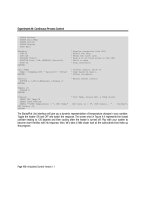
accordingly. A typical block diagram of an automatic control system is depicted in Figure 5.1.

Experiment #5:
Closed-Loop
Control

Figure 5.1: Closed-Loop Control

In this diagram, an appropriate sensor is measuring the Actual Output. The signal-conditioning block takes the
raw output of the sensor and converts it into data for the Controller block. The Setpoint is an input to the
Controller block that represents the desired output of the process. The controller evaluates the two pieces of
data. Based on this evaluation, the controller initiates action on the Power Interface. This block provides the
signal conditioning at the controller’s output. Experiment #3 discussed several methods of driving power
interface circuits. The Power Interface has the ability to control the Actuator. This may be a relay, a solenoid
valve, a motor drive, etc. The action taken by the Actuator is sufficient to drive the Actual Output toward the
desired value.


Industrial Control Version 1.1 • Page 127


Experiment #5: Closed-Loop Control

As you can see, this control scenario forms a loop, a closed-loop. Furthermore, since it is the process’s output
that is being measured, and its value determines actuator settings, it is a feedback closed-loop system. The
input changes the process output
the output is monitored for evaluation
the evaluation changes the
input that changes the process output, etc., etc.
The type of reaction that takes place upon evaluation of the input defines the process-control mode. There
are five common control modes. They are on-off, on-off with differential gap, proportional, integral, and
derivative. The fundamental characteristic that distinguishes each control mode is listed below in Table 5.1.
Table 5.1: Five Common Control Modes
Process
Control Mode
On-off

Integral

Evaluation
Is the variable above or below a
specific desired value?
Is the variable above or below a range
defined by an upper and lower limit?
How far is the measured variable away
from the desired value?
Does the error still persist?


Derivative

How fast is the error occurring?

On-off with
differential gap
Proportional

Action
Drive the output fully ON or fully OFF.
Output is turned fully ON and fully OFF to drive
the measured value through a range.
Take a degree of action relative to the
magnitude of the error.
Continue taking more forceful action for the
duration the error exists.
Take action based on the rate at which the
error is occurring.

Continue taking more forceful action for the duration the error exists.
This exercise will focus on converting the open-loop temperature control system of Experiment #4 into an
on-off closed-loop system. Our system will show advantages and disadvantages to this method of control. The
characteristics of the system being controlled determines how suitable a particular control mode will be.
Experiment #6 will use the same circuitry to overview and apply proportional, integral, and derivative control
modes. Leave the circuit constructed after completing this step.
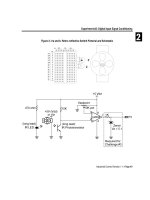
Figure 5.2 is a schematic of the circuitry necessary for the next two exercises. As you see, this is identical to
Experiment #4. The 35-mm film canister provides the environment we wish to control. The heater drive
provides full power for developing heat in the resistor. The LED is also driven by Pin 8. Remember that the LED
is driven by the +5-Vdd supply, and the heater is driven by the +9-volt unregulated line supply. The LM34
sensor will provide temperature data. In closed-loop control, we will monitor the temperature and use it to

determine control levels. The fan’s air currents will act as a disturbance to the process.

Page 128 • Industrial Control Version 1.1


Experiment #5: Closed-Loop Control

Figure 5.2: Closed-Loop Control Circuitry

Industrial Control Version 1.1 • Page 129


Experiment #5: Closed-Loop Control

If the circuit isn’t already on your board, carefully construct it. Use space on the small Board of Education
efficiently to allow for the circuitry. Take your time, plan your layout, and be careful not to inadvertently short
any wires. Refer back to Experiment #4 for details on the film canister construction, the operation of the
LM34, and the use of the ADC0831 analog-to-digital converter.
Double-check the Zero and Span voltages of the ADC0831. Use your voltmeter to set the Zero voltage (Vin(-))
to .7 and the Span (V(ref)) to .5 volts. This will establish a full-scale temperature measurement range from 70
to 120 degrees F.

Exercises

Exercise #1: Establishing Closed-Loop Control
Let’s assume it is our objective to maintain temperature within the canister at 101.50 oF + 1 degree. This
would be representative of the requirements of an incubator used for hatching eggs. Maintaining the eggs at
the setpoint temperature of 101.5 oF is perfect, but the temperature could go up to 102.50 or down to 100.50
without damage to the embryos. Although it may be hard to imagine an incubator when you look at your film
canister, the BASIC Stamp would be well suited as the controller in a large commercial hatchery incubator.

To maintain temperature at the desired value seems like a pretty “common sense” task. That is, simply
measure temperature; if it is above the setpoint, turn the heater OFF; and, if it is below, turn the heater ON.
The simplest kind of control mode is on-off control. There are drawbacks to this control mode, however.
During the following exercise, you will establish on-off control of your model incubator. Pay close attention to
the characteristics exhibited by your model. These characteristics would also apply to real control
applications.
Procedure
Programming for this application requires data acquisition, evaluation, and control action. Our display routine
will also include storing and displaying the minimum and maximum overshoot in the process.
The structure and much of the content of Program 4.1 may be used to acquire and calculate our
measurement. Instead of turning the heater on continually, a new subroutine will be added to evaluate and
control it. Evaluation will be based on a setpoint variable. Refer to Program 5.1 following.

Page 130 • Industrial Control Version 1.1