143
Ann. For. Sci. 62 (2005) 143–152
© INRA, EDP Sciences, 2005
DOI: 10.1051/forest:2005006
Original article
Site quality equations for Pinus sylvestris L. plantations in Galicia
(northwestern Spain)
Ulises DIÉGUEZ-ARANDA*, Juan Gabriel ÁLVAREZ GONZÁLEZ, Marcos BARRIO ANTA,
Alberto ROJO ALBORECA
Departamento de Ingeniería Agroforestal, Universidad de Santiago de Compostela, Escuela Politécnica Superior,
Campus universitario, 27002 Lugo, Spain
(Received 17 May 2004; accepted 18 October 2004)
Abstract – Difference equations derived on the basis of the Sloboda and McDill-Amateis differential functions, and from the integral form of
the Bertalanffy-Richards, Korf and Hossfeld growth functions were used to model the dominant height growth of Scots pine (Pinus sylvestris
L.) in Galicia (north-western Spain). Data from stem analysis and permanent sample plots were combined and used for fitting. Both numerical
and graphical analyses were used to compare alternative models. The cross-validation approach was used to analyse the predictive ability of
the models. The algebraic difference form of the differential function proposed by McDill and Amateis resulted in the best compromise between
biological and statistical aspects, producing the most adequate site curves. It is therefore recommended for height growth prediction and site
classification of Scots pine plantations in Galicia. This equation is base-age invariant, so any number of points (A
1
, H
1
) on a specific site curve
can be used to make predictions for a given age A
2
and the predicted height H
2
will always be the same.
height growth / site classification / algebraic difference equation / even-aged forest stand
Résumé – Équations prédictives de la fertilité des stations pour des plantations de Pinus sylvestris L. en Galice (nord-ouest de
l’Espagne). À partir des équations différentielles de Sloboda et McDill-Amateis, ainsi que de la forme intégrale de Bertalanffy-Richards, Korf

et Hossfeld, un modèle a été établi pour caractériser la croissance en hauteur dominante du pin sylvestre (Pinus sylvestris L.) en Galice (nord-
est de l’Espagne). Des données, issues à la fois de l’analyse de tiges et de l’accroissement de placettes semi-permanentes, ont été combinées
pour établir ce modèle. Des analyses numériques et graphiques ont été utilisées pour comparer les différents modèles existants. Les résidus de
la validation croisée ont été utilisés pour évaluer le comportement des équations. L’équation en différences algébriques obtenue à partir de la
fonction différentielle de McDill et Amateis donna le meilleur compromis entre les aspects biologique et statistique, fournissant les courbes de
qualité les plus adéquates. C’est donc l’équation recommandée pour prédire la croissance en hauteur et pour réaliser les classifications de qualité
des sites de plantation des pins sylvestres en Galice. Cette équation est invariante quant à l’âge de référence, de sorte que la hauteur à un âge
donné peut être estimée à partir de la hauteur à un autre âge, sans compromettre la validité des prédictions.
croissance en hauteur / classement des sites / équation en différence algébrique / peuplement équienne
1. INTRODUCTION
The classification of forest land in terms of its productivity
is an important issue for forestry managers, as well as for for-
estry enterprise administrators. An index which expresses this
productivity is a required variable for the modelling of present
and future growth and yield, and can also be used for forest land
stratification for purposes of forest inventory, and for forest
exploitation on a sustainable yield basis [24].
Conceptually, site quality is considered an inherent property
of plots of land, whether or not trees are being grown at the time
of interest. The productivity of specific stand can vary greatly
due to a host of factors including the underlying soil conditions,
climatic variables and management practices. For timber pro-
duction purposes, and especially for even-aged forest stands,
site quality is commonly expressed as a species-specific site
index [14, 21]. Site index may be defined as height, at a prede-
termined age, of dominant or codominant trees that have always
been dominant or codominant and healthy [29]. Empirical evi-
dence from thinning experiments indicates that for many commer-
cially important species, height growth is not greatly affected
by the manipulation of stand density. However, the average

height of the stand may be affected by thinning, depending on
the method used, but within limits of stand density, height
growth appears to be unaffected, particularly when the com-
parison is restricted to dominant and codominant trees [20].
* Corresponding author:
144 U. Diéguez-Aranda et al.
Site quality associated with Scots pine (Pinus sylvestris L.)
in Spain has been studied by several authors. The earliest site
index curves were constructed using methods that could all be
classified within the guide curve method [25–27, 41, 47, 51].
All of these studies together covered the three main areas of dis-
tribution of the species in Spain: the Sistema Central Moun-
tains, the Sistema Ibérico Mountains and the Pyrenees. A further
description of studies related to site quality of Scots pine up to
1996 is provided by Rojo and Montero [51]. More recently,
Bravo and Montero [7] developed a system for site index esti-
mation for this species in the High Ebro Basin (northern Spain),
by considering soil attributes and using an extension of the
Richards’ model. Finally, Palahí et al. [44] developed a site
quality system for Scots pine in the northeast of Spain using
data from permanent plots and stem analysis. These authors
tested eleven equations for modelling dominant height growth.
Most of the equations were derived from functions frequently
used in forest growth modelling, by means of the algebraic dif-
ference approach [5, 12, 20, 37] and the generalized algebraic
difference approach [18]. Other recent studies related to growth
and yield of Scots pine in Spain are from Palahí et al. [43], Palahí
and Pukkala [42], Bravo and Montero [8], and Bravo and Díaz-
Balteiro [6].
The objective of the present study was to develop a site index

system for pure Scots pine plantations in Galicia (northwest of
Spain).
2. MATERIALS AND METHODS
2.1. Data
The data used to develop the site index curves were obtained from
two different sources. Initially, in the winter of 1996 and 1997 a net-
work of 185 plots was established in pure Scots pine plantations. The
plots were located throughout the area of distribution of this species
in Galicia, and were subjectively selected to represent the existing
range of ages, stand densities and sites. The plot size ranged from
625 m
2
to 1200 m
2
, depending on stand density, in order to achieve a
minimum of 60 trees per plot. We adopted this procedure because the
plots were established for developing a whole stand model and an ade-
quate number of trees is required to accurately estimate yield and
growth. Two dominant trees were destructively sampled at 118 loca-
tions. These trees were selected as the first two dominant trees found
outside the plots but in the same stands within ± 5% of the mean diam-
eter at 1.3 m above ground level and mean height of the dominant trees
(considered as the 100 largest-diameter trees per hectare). The trees
were felled leaving stumps of average height 0.11 m; total bole length
was measured to the nearest 0.01 m. The logs were cut at 2 to 2.5 m
intervals for the first 4 to 5 m of bole length and at 1 m intervals there-
after. Number of rings was counted at each cross-sectioned point, and
then converted to stump age, which can be considered equal to plan-
tation age. As cross section lengths do not coincide with periodic
height growth, it was necessary to adjust height/age data from stem

analysis to account for this bias using Carmean’s method [13], and the
modification proposed by Newberry [40] for the topmost section of
the tree. A test of six methods of estimating true heights from stem
analysis data [22] showed that Carmean’s algorithm provided the most
accurate estimates. The data of these 236 stem analyses composed the
first source of data.
A subset of 79 of the above-mentioned plots was re-measured in
the winter of 2003. These plots were selected for developing a dynamic
growth model for the species in the area of study, thus the initial
number of plots installed in 1996–1997 was considerably reduced
because the plots measured twice provided better information con-
cerning the development of Scots pine stands. The dominant height
of each of these plots was calculated as the mean height of the
100 thickest trees per hectare, both for the first and the second inven-
tories. The data on age (excluding seedling age for plantation) and
dominant height in these plots measured twice constituted the second
source of data used in the study.
Summary statistics including number of observations, mean, stand-
ard deviation, minimum, and maximum values were calculated for the
total tree height and plot dominant height variables grouped by age
classes (Tab. I). All the data were converted to a two-year interval
structure (i.e. heights for ages at 2, 4, 6, etc. years) using Carmean’s
algorithm (in the case of trees) or interpolating between the observed
heights at the ages of measurement for the plots.
2.2. Methods for constructing a site index system
According to Clutter et al. [20], most techniques for site index
curves construction can be viewed as special cases of three general
methods: (1) the guide curve method, (2) the parameter prediction
method, and (3) the difference equation method. Although the three
methods are not mutually exclusive, the difference equation method

has been the preferred form for developing site index curves [1, 2, 5,
11, 45, 48].
The difference equation method makes direct use of the fact that
observations corresponding to a given plot or dominant tree should
belong to the same site curve. A height-by-age equation can be differ-
entiated to provide an equation for height growth rather than accumulated
height. An equation in this form is referred to as an algebraic difference
equation [45]. In this method, height H
2
at age A
2
is expressed as a
function of A
2
, height H
1
at age A
1
and A
1
. The expression is obtained
through substitution of one parameter in the growth model. The choice
of this parameter determines the behaviour of the model, which is
capable of producing anamorphic or polymorphic (with single asymp-
tote) curve families.
With the difference equation method (1) short observation periods
of temporary plots or stem analysis from trees whose total age is under
or over the reference age can be used, (2) the curves pass through site
index at the reference age, and (3) they are base-age invariant [19, 20].
The invariant or unchanging property refers to predicted heights: any

number of points (A
1
, H
1
) on a specific site curve can be used to make
predictions for a given age A
2
and the predicted height H
2
will always
be the same. This includes forward and backward predictions, and the
path invariance property that ensures the result of projecting first from
A
1
to A
2
, and then from A
2
to A
3
, being the same as that of the one-
step projection from A
1
to A
3
. Equations derived using this technique
define both height-growth and site index models as special cases of
the same equation [16].
Table I. Total tree height or plot dominant height statistics, given in
meters (age class 15 = 10–19 years, etc.).

Age class Number
of obs.
Mean Standard
deviation
Minimum
value
Maximum
value
15 18 6.11 1.41 4.2 8.6
25 53 8.56 2.84 4.6 17.3
35 162 11.47 3.40 4.8 20.5
45 69 15.65 4.21 6.6 24.0
55 7 17.13 3.57 9.8 20.1
65 4 20.45 2.49 17.7 23.1
75 2 26.71 0.20 26.6 26.9
Site quality of Pinus sylvestris L. in Galicia 145
2.3. Function selection
Growth functions describe variations in the global size of an organ-
ism or a population with age; they can also describe the changes in a
particular variable of a tree or a stand with age, in this case dominant
height.
There are many growth functions that can be employed in forestry,
such as the 74 documented by Kiviste et al. [35]. The most important
desirable attributes for site index equations are: (1) polymorphism,
(2) sigmoid growth pattern with an inflexion point, (3) horizontal
asymptote at old ages, (4) logical behaviour (height should be zero at
age zero and equal to site index at the reference age), and (5) base-age
invariance [2, 28, 45]. The fulfilment of these attributes depends on
both the construction method and the mathematical function used to
develop the curves, and it cannot always be achieved.

Multiple asymptotes (i.e. asymptote varying with site index, typi-
cally higher site indices having higher asymptotes) may also be a desir-
able attribute [15, 18], although some of the frequently used functions
have a common asymptote. This does not appear to be of great impor-
tance, as the behaviour of the curves is generally suitable for the range
of ages that would be used in practice, and the common asymptote is
usually achieved at very old ages. Limits for usage must always be
appended to the curves [28].
A total of seven models were selected for fitting the height/age rela-
tionship (Tab. II). The first six models were derived using the differ-
ence equation method. Models M1 and M2 were formulated on the
basis of the differential equations proposed by Sloboda [53] and
McDill and Amateis [37], respectively. Models M3 to M6 were for-
mulated from the integral form of the Bertalanffy-Richards model [3,
4, 50]; and based on the integral form of Korf’s model (cited in [36]).
Table II. Algebraic difference models considered.
Model Algebraic difference model Base equation
M1
Sloboda [53]
M2
McDill and Amateis [37]
M3
Bertalanffy-Richards
solved by b
1
M4
Bertalanffy-Richards
solved by b
2
M5

Korf
solved by b
1
M6
Korf
solved by b
2
M7
with and
Hossfeld IV
solved by b
0
and assuming
b
1
= b
3
/S
H
1
and H
2
are dominant height (m) at ages A
1
and A
2
(years), respectively; Asi is an age between 5 and 50 years used to reduce the mean square error;
ln is the natural logarithm; and b
0
, b

1
, b
2
and b
3
are parameters to be estimated.
H
2
b
0
H
1
b
0



e
b
1
b
2
1–()A
2
b
2
1–()

b
1

b
2
1–()A
1
b
2
1–()

–





=
dH
dA

b
0
H



b
1
H
A
b
2





ln=
H
2
b
0
11
b
0
H
1
–


A
1
A
2



b
1
–
=
dH
dA

1
H
b
0
–


b
1
H
A

=
H
2
b
0
11
H
1
b
0



1
b
2

–





A
2
A
1

–






b
2
=
Hb
0
1 e
b
1
A–
–()
b
2
=
H

2
b
0
H
1
b
0



1 e
b
1
A
2
–
–


ln
1 e
b
1
A
1
–
–


ln


=
Hb
0
1 e
b
1
A–
–()
b
2
=
H
2
b
0
H
1
b
0



A
1
A
2




b
2
=
Hb
0
e
b
1
A
b
2
–
–
=
H
2
b
0
b
1
– A
2
H
1
/b
0
()ln
b
1
–




/
A
1
lnln






exp=
Hb
0
e
b
1
A
b
2
–
–
=
H
2
H
1
dr++

2
4b
3
A
2
b
2
H
1
dr+–()
+
=
d
b
3
Asi
b
2
= rH
1
d–()
2
4b
3
H
1
A
1
b
2

–
+=
H
b
0
1
b
1
A
b
2
+
=
146 U. Diéguez-Aranda et al.
Model M7 was proposed by Cieszewski and Bella [19] from the Hoss-
feld IV equation (cited in [46]) by relating a model parameter to site index.
The approach used to derive model M7 can be referred to as initial-
condition site index substitution in expanded dynamic equations [17].
These algebraic difference equations are base-age invariant, poly-
morphic, and model M7 has multiple asymptotes. All the models have
been widely used to develop height/age curves [10, 19, 23, 24, 54].
2.4. Data structure and model fitting
The data structure used for fitting the seven models was arranged
with all the possible combinations among height/age pairs for each tree
and plot, including descending growth intervals. All possible growth
intervals typically produce fitted models with a better predictive per-
formance as compared to, for example, forward moving first differ-
ences [28, 32]. However, this data structure may lead to the rejection
of the error assumptions because it automatically introduces a lack of
independence among observations [28]. Although under noninde-

pendence the parameter estimates are even unbiased, standard error
estimators are biased [30].
The potential problem of lack of independence among observations
and heteroscedasticity can be solved using generalised nonlinear least
squares (GNLS) methods [28, 31, 38]. In this case, autocorrelation was
modelled by expanding the error term in the following way [28, 29, 45]:
H
ij
= f(H
j
, A
i
, A
j
, β) + e
ij
with e
ij
= ρe
i–1
,
j
+ γ e
i,j–1
+ ε
ij
(1)
where H
ij
depicts prediction of height i by using H

j
(height j), A
i
(age i),
and A
j
(age j ≠ i) as predictor variables; β is the vector of parameters
to be estimated; e
ij
is the corresponding error term; the ρ parameter
accounts for the autocorrelation between the current residual and the
residual from estimating H
i–1
using H
j
as a predictor; the γ parameter
accounts for the autocorrelation between the current residual and the
residual from estimating H
i
using H
j–1
as a predictor; and ε
ij
are inde-
pendent and identically distributed errors.
To avoid the possible problem of heteroscedasticity, the variance
of errors was assumed to be a power function of the predicted dominant
height [32, 33]. The weighting factors used were ,
where k is a constant. Since the predicted dominant heights are initially
unknown, different values of k (e.g. k = –0.4, –0.2, 0, 0.2, 0.4) were

tested until heteroscedasticity was corrected.
In using all possible differences, the number of observations is arti-
ficially inflated and the corresponding standard errors for the param-
eters are therefore too small. Thus, the standard errors were expanded
by , where n(apd) is the number of observations using
all possible differences and n(fd) is the number of observations if using
only first differences [29].
Fitting was carried out by modelling the mean and the error struc-
ture simultaneously, using the SAS/ETS

MODEL procedure [52].
This method of proceeding simultaneously optimizes the regression
of H on A and A on H, and avoids parameter bias due to independent
estimation of (1) site index at base age given height at some other age,
and (2) height at some desired age given height (site index) at base
age [28, 29, 45].
For model M7, the parameter Asi was ranged from 5 to 50 years in
order to reduce the mean square error [23, 54].
2.5. Model comparison and model selection
The comparison of the estimates of the eight models fitted for pre-
dicting dominant height over age was based on numerical and graph-
ical analyses. Three statistical criteria obtained from the residuals were
examined: root mean square error (RMSE), which analyses the accu-
racy of the estimates; the adjusted coefficient of determination (R
2
adj
),
which shows the proportion of the total variance that is explained by
the model, adjusted for the number of model parameters and the
number of observations; and Akaike’s information criterion differ-

ences (AICd), which is an index for selecting the best model on the
basis of minimizing the Kullback-Liebler distance [9]. Their expres-
sions may be summarized as follows:
(2)
(3)
(4)
where , and are the measured, predicted and average values
of the dependent variable, respectively; n is the total number of obser-
vations used to fit the model; p is the number of model parameters;
k = p + 1; and is the estimator of the error variance of the model
obtained with the following equation:
(5)
The cross-validation of each model was based on the analysis of
root mean square error of the estimates, the adjusted model efficiency
(ME
adj
, equivalent to the R
2
adj
of the previous phase), and the Akaike’s
information criterion differences, obtaining the residual of each tree
or plot by refitting the model without that tree or plot.
Apart from these three statistics, one of the most efficient ways of
ascertaining the overall picture of model performance is by visual
inspection, so graphical analyses consisting of plots of observed
against predicted values of the dependent variable and plots of studen-
tized residuals against the predicted dominant height were carried out.
These graphs are useful both for detection of possible systematic dis-
crepancies and for selecting the weighting factor [39]. Additionally,
graphs showing the appearance of the fitted curves overlaid on the tra-

jectories of the stem analysis or plot data over time were examined.
Practical use of the models to estimate site quality from any given
pair of height and age requires the selection of a base age to which
site index will be referenced. Inversely, site index and its associated
base age could be used to estimate dominant height at any desired age.
Selection of the base age for the site index equations was made accord-
ing to the following considerations [28]: (1) the base age should be
less than or equal to the youngest rotation age under typical management,
(2) the base age should be close to the rotation age, and (3) the base age
should be chosen so that it is a reliable predictor of height at other ages.
In order to address the third consideration, different base ages and
their corresponding observed heights were used to estimate heights at
other ages for each tree or plot. The results were compared with the
values obtained from stem analyses and plot re-measurements, and the
relative error in predictions (RE%) was then calculated as follows:
(6)
where , and are the measured, predicted and average values
of the dependent variable, respectively; n is the total number of obser-
vations used to fit the model; and p is the number of model parameters.
w
i
pred.H
i
k
=
n apd()/n fd(
)
RMSE
y
i

y
ˆ
i
–()
2
i 1=
n
∑
np–
=
R
adj
2
1
n 1–()y
i
y
ˆ
i
–()
2
i 1=
n
∑
np–()y
i
y–()
2
i 1=
n

∑
–=
AICd n
σ
ˆ
2
log 2k min n

σ
ˆ
2
log 2k+()–+=
y
i
y
ˆ
i
y
σ
ˆ
2
σ
ˆ
2
y
i
y
ˆ
i
–()

2
i 1=
n
∑
n

.
=
RE%
y
i
y
ˆ
i
–()
2
i 1=
n
∑
/ np–()
y

100=
y
i
y
ˆ
i
y
Site quality of Pinus sylvestris L. in Galicia 147

In addition to the graphs mentioned above, and because by defini-
tion site index is a fixed stand attribute that should be stable over time
[32, 38], graphs showing the stability or the consistency of site index
predictions over time were also constructed.
Finally, H
2
at A
2
was estimated considering previous H
1
at A
1
as
predictors, and using different intervals of 2, 4, 6, etc. years, in order
to find out for how long the estimations could be made from any given
pair of height and age. Root mean square error over age was calculated
for different age lags. For each of the different lags tested, a critical
error (E
crit.
) expressed as a percentage of the observed mean was also
computed by re-arranging Freese’s statistic [49]:
(7)
where n is the total number of observations in the data set, y
i
is the
observed value, is its prediction from the fitted model, is the aver-
age of the observed values, τ is a standard normal deviate at the spec-
ified probability level (τ = 1.96 for α = 0.05), and is obtained
for and n degrees of freedom. If the specified allowable error,
expressed as a percentage of the observed mean, is within the limit of

the critical error, the test will indicate that the model does not give
satisfactory predictions; otherwise, it will indicate that the predictions
are acceptable.
3. RESULTS AND DISCUSSION
The parameter estimates for each model and the statistics for
both the fitting and the cross-validation phases are shown in
Table III. All the parameters were found to be significant at a 5%
level when the expansion factor proposed by [29] was applied.
In general, weightings factors of and
showed the best results when plots of stu-
dentized residuals against the predicted heights were examined for
detection of possible systematic trends of unequal error variance.
The values of the statistics used to compare the models indi-
cate that all the models, except model M6 (Korf solved by b
2
),
produced a reasonable performance with low RMSE for fitting
and cross-validation. These results suggest that, for this spe-
cies, the indicated solution of Korf’s model is not suitable for
modelling the height/age relationship, as the b
2
parameter
does not depend on site quality. Similar results were obtained
by [1]. The best results for model M7 [19] were obtained
when Asi = 30 was used. Models M1 (Sloboda [53]) and M4
(Bertalanffy-Richards solved by b
2
) provided the best results
for the goodness-of-fit statistics calculated, although models
M2 (McDill and Amateis [37]) and M3 (Bertalanffy-Richards

solved by b
1
) represented the data almost as well, with both
behaving similarly. Thereafter, the selection of the best model
focused on these four models.
As previously commented, visual or graphical inspection of
the models is considered an essential point in selecting the most
accurate representation. Therefore, plots showing the site
curves for heights of 5, 10, 15 and 20 m at 40 years overlaid
on the trajectories of observed values over time (Fig. 1) were
examined. They indicated that at young ages models M1 (Sloboda
[53]) and M4 (Bertalanffy-Richards solved by b
2
) overestimated
Figure 1. Plots showing the site curves for heights of 5, 10, 15 and 20 m at 40 years overlaid on the trajectories of observed values over time.
χ
n
2
E
crit.
τ
2
y
i
y
ˆ
i
–()
2
i 1=

n
∑
/χ
crit.
2
y
=
y
ˆ
i
y
χ
crit.
2
α 0.05=
χ
n
2
w
i
1/pred.H
i
0.2
=
w
i
1/pred.H
i
0.4
=

148 U. Diéguez-Aranda et al.
heights for the best sites and underestimated heights for the
poorest sites. At older ages the curves generated from these
models seem to increase quicker than the trajectories of trees
and plots show.
In selecting the base age, it was found that a base age of 40
to 45 years was superior for predicting height at other ages with
a minimum of reliability (Fig. 2). Even though at older ages the
relative error in predicting height was lower, the scarcity of data
Table III. Parameter estimates and statistics for model comparison.
Model Parameters Approx.
expanded
std. error
Fitting Cross-validation
RMSE R
2
adj
AICd RMSE ME
adj
AICd
b
0
67.90 2.53
0.484 0.9912 0 0.949 0.9662 0
b
1
0.1571 0.002
b
2
0.6179 0.009

ρ 0.9276 0.013
γ 0.1358 0.011
M2
b
0
51.39 0.97
0.527 0.9896 11659 1.029 0.9603 11153
b
1
1.277 0.004
ρ 0.9693 0.011
γ 0.1032 0.010
M3
b
0
37.90 0.61
0.528 0.9895 12021 1.031 0.9601 11469
b
2
1.294 0.005
ρ 0.9689 0.011
γ 0.1035 0.010
M4
b
0
64.22 1.91
0.501 0.9906 4798 0.984 0.9637 5012
b
1
0.008475 0.000

ρ 0.9410 0.012
γ 0.1232 0.011
M5
b
0
19438 4608
0.589 0.9870 27161 1.188 0.9470 30925
b
2
0.1323 0.004
ρ 0.9767 0.011
γ 0.09856 0.010
M6
b
0
158.1 11.6
1.125 0.9525 116067 2.242 0.8115 118258
b
1
7.034 0.057
ρ 1.041 0.008
γ 0.04942 0.007
M7
b
2
1.262 0.004
0.542 0.9890 15757 1.068 0.9572 16281
b
3
3116 55

Asi 30 –
ρ 0.9707 0.011
γ 0.1030 0.010
Site quality of Pinus sylvestris L. in Galicia 149
would lead to an incorrect decision as the data were not repre-
sentative enough (less than 30 trees or plots). According to
[28], this selection procedure should be devised so that variance
of the volume estimates for the forest of interest are minimized,
which requires that site index equations be integrated in a
growth and yield system. Nevertheless, the lack of necessary
information forced us to conclude that a reference age of
40 years is appropriate for Scots pine in Galicia.
The present investigation was based primarily on trees with
a height at 40 years of between 6–22 m. Some of the trees were
older than 55 years. Taking into account that most of the stands
of the type covered in this study will be clear-felled at around
80–100 years, curves for heights up to 80 years were con-
structed. However, the use of the curves should always be
approached with caution for ages above 60 years. Moreover,
curves should be used for ages greater than 10 years, since for
younger ages the erratic behaviour of the trees at initial ages
may lead to erroneous classifications.
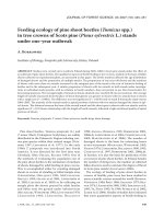
Finally, plots showing the stability of site index predictions
over time (Fig. 3) show that models M2 (McDill and Amateis
[37]) and M3 (Bertalanffy-Richards solved by b
1
) provided the
best results, judged by the consistency of predicted values over
time. These two models performed adequately (taking into
account numerical and graphical criteria) and both would be

suitable for developing a site index system.
Summing up, model selection has been viewed as a com-
promise between biological and statistical considerations.
Model M2 – the algebraic difference form of the differential
function proposed by McDill and Amateis [37] – produced
curves with an adequate graphical behaviour as well as good
values of the goodness-of-fit statistics. Based on these consid-
erations, we propose its use for height growth prediction and
site classification of Scots pine stands in Galicia:
(8)
where H
1
and A
1
represent the predictor height (meters) and age
(years), and H
2
is the predicted height at age A
2
.
It should be noted that model M2 is parsimonious, as it
includes only two parameters (excluding the correlation ones),
and fits the data as well as, or better than, other models that were
tried.
To use model M2 to estimate average stand height (H) for
some desired age (A), given site index (S) and its associated
base age (A
b
), substitute S for H
1

and A
b
for A
1
in equation (8):
.
(9)
Similarly, to estimate site index at some chosen base age,
given stand height and age, substitute S for H
2
and A
b
for A
2
in equation (8):
.
(10)
As regards how long the curves should be used for estimating
height at any age given height at any other age, the plot of RMSE
Figure 2. Relative error in height predictions related to choice of reference age. Ages older than 44 years are not representative enough due to
the lack of data.
H
2
51.39
11
51.39
H
1
–



A
1
A
2



1.277
–
=
H
51.39
11
51.39
S
–


A
b
A



1.277
–
=
S
51.39

11
51.39
H
–


A
A
b



1.277
–
=
150 U. Diéguez-Aranda et al.
against age for different year lags (Fig. 4 left) shows that as lag
increases RMSE also increases for all ages, being more or less
stable over time for the ages where enough data are available,
and is, e.g. a maximum of 1 m for lag = 8 years and 1.8 m for
lag = 20 years. From the plot showing the critical error against
different year lags (Fig. 4 right), it can be observed that for lags
of more than eight years the critical error exceeded 20%. In both
cases, and for either ages or lags of more than 40–45 years, the
calculated statistics are not reliable because of a lack of data.
Considering the required accuracy in forestry growth modelling,
where a mean prediction error of the observed mean at 95%
confidence intervals within ± 10%–20% is generally realistic
and reasonable as a limit for the actual choice of the acceptance
and rejection levels [34], it can be stated that projections of

dominant height should not be made directly for differences in
age of more than eight years; that is, for a given stand, projec-
tions of more than this length of time should be tested with real
data as time passes, and these new data should be used to make
new projections.
4. CONCLUSIONS
In practical terms, equation (8) is recommended for height
growth prediction and site classification in the age interval 10–
60 years in Scots pine plantations in Galicia, although the
curves could also be used with caution for ages up to 70–
80 years. It is also recommended that field studies of height
growth in old pine plantations are continued.
Figure 3. Site index predictions against total age using the stem analysis data and the data of the plots measured twice.
Figure 4. Plot of RMSE against age for different year lags (left) and plot of critical error against different year lags (right) for model M2.
Site quality of Pinus sylvestris L. in Galicia 151
Equation (8) can be solved for any base age, so estimates of
Scots pine stand height and site index are easily obtained
through direct evaluation of the function; there is no need for
iterative numerical evaluation methods.
Visual inspection of the models is essential because numer-
ical analyses may provide the best results for models that do
not fit the data well enough.
Finally, it should be noted that projections of dominant
height should not be made directly for differences in age of
more than eight years, i.e. for a given stand, projections of more
than this length of time should be tested with real data as time
passes, and these new data should be used to make new pro-
jections.
Acknowledgements: The authors express their appreciation to Dr.
Timothy G. Gregoire and one anonymous reviewer for their valuable

suggestions. Funding for this research was provided by the Ministry
of Science and Technology through project AGL2001-3871-C02-01
“Crecimiento y evolución de masas de pinar en Galicia”.
REFERENCES
[1] Álvarez González J.G., Ruiz González A.D., Rodríguez Soalleiro
R.J., Barrio Anta M., Development of ecoregion-based site index
models for even-aged stands of Pinus pinaster Ait. in Galicia (north-
western Spain), Ann. For. Sci. 62 (2005) 117–129.
[2] Bailey R.L., Clutter J.L., Base-age invariant polymorphic site cur-
ves, For. Sci. 20 (1974) 155–159.
[3] Bertalanffy L.v., Problems of organic growth, Nature 163 (1949)
156–158.
[4] Bertalanffy L.v., Quantitative laws in metabolism and growth, Q.
Rev. Biol. 32 (1957) 217–231.
[5] Borders T.H., Bailey R.L., Ware K.D., Slash pine site index from a
polymorphic model by joining (splining) nonpolynomial segments
with an algebraic difference method, For. Sci. 30 (1984) 411–423.
[6] Bravo F., Díaz-Balteiro L., Evaluation of new silvicultural alterna-
tives for Scots pine stands in northern Spain, Ann. For. Sci. 61
(2004) 163–169.
[7] Bravo F., Montero G., Site index estimation in Scots pine (Pinus
sylvestris L.) stands in the High Ebro Basin (northern Spain) using
soil attributes, Forestry 74 (2001) 395–406.
[8] Bravo F., Montero G., High-grading effects on Scots pine volume
and basal area in pure stands in northern Spain, Ann. For. Sci. 60
(2003) 11–18.
[9] Burnham K.P., Anderson D.R., Model selection and inference. A
practical information-theoretic approach, Springer-Verlag, New
York, 1998.
[10] Calama R., Cañadas N., Montero G., Inter-regional variability in

site index models for even-aged stands of stone pine (Pinus pinea
L.) in Spain, Ann. For. Sci. 60 (2003) 259–269.
[11] Cao Q.V., Estimating coefficients of base-age invariant site index
equations, Can. J. For. Res. 23 (1993) 2343–2347.
[12] Cao Q.V., Baldwin V.C., Lohrey R.E., Site index curves for direct-
seeded loblolly and longleaf pines in Lousinia, North J. Appl. For.
21 (1997) 134–138.
[13] Carmean W.H., Site index curves for upland oaks in the central sta-
tes, For. Sci. 18 (1972) 109–120.
[14] Carmean W.H., Forest site quality evaluation in the United States,
Adv. Agron. 27 (1975) 209–267.
[15] Cieszewski C.J., Comparing fixed-and variable-base-age site equa-
tions having single versus multiple asymptotes, For. Sci. 48 (2002)
7–23.
[16] Cieszewski C.J., Developing a well-behaved dynamic site equation
using a modified Hossfeld IV function Y
3
=(ax
m
)/(c + x
m–1
), a sim-
plified mixed-model and scant subalpine fir data, For. Sci. 49
(2003) 539–554.
[17] Cieszewski C.J., Bailey R.L., The method for deriving theory-
based base-age invariant polymorphic site equations with variable
asymptotes and other inventory projection models, University of
Georgia, PMRC Technical Report 1999–4.
[18] Cieszewski C.J., Bailey R.L., Generalized algebraic difference
approach: theory based derivation of dynamic equations with poly-

morphism and variable asymptotes, For. Sci. 46 (2000) 116–126.
[19] Cieszewski C.J., Bella I.E., Polymorphic height and site index cur-
ves for lodgepole pine in Alberta, Can. J. For. Res. 19 (1989) 1151–
1160.
[20] Clutter J.L., Fortson J.C., Pienaar L.V., Brister G.H., Bailey R.L.,
Timber management: a quantitative approach, Krieger Publishing
Company, New York, 1983, Reprint ed. 1992.
[21] Davis L.S., Johnson K.N., Bettinger P.S., Howard T.E., Forest
management: to sustain ecological, economic, and social values,
McGraw-Hill, New York, 2001.
[22] Dyer M.E., Bailey R.L., A test of six methods for estimating true
heights from stem analysis data, For. Sci. 33 (1987) 3–13.
[23] Elfving B., Kiviste A., Construction of site index equations for
Pinus sylvestris L. using permanent plot data in Sweden, For. Ecol.
Manage. 98 (1997) 125–134.
[24] García O., A stochastic differential equation model for the height
growth of forest stands, Biometrics 39 (1983) 1059–1072.
[25] García Abejón J.L., Tablas de producción de densidad variable para
Pinus sylvestris en el Sistema Ibérico, Comunicaciones INIA Serie:
Recursos Naturales, nº 10, 1981.
[26] García Abejón J.L., Gómez Loranca J.A., Tablas de producción de
densidad variable para Pinus sylvestris en el sistema Central,
Comunicaciones INIA Serie: Recursos Naturales, nº 29, 1984.
[27] García Abejón J.L., Tella G., Tablas de producción de densidad
variable para Pinus sylvestris L. en el Sistema Pirenaico, Comuni-
caciones INIA Serie: Recursos Naturales, nº 43, 1986.
[28] Goelz J.C.G., Burk T.E., Development of a well-behaved site index
equation: jack pine in north central Ontario, Can. J. For. Res. 22
(1992) 776–784.
[29] Goelz J.C.G., Burk T.E., Measurement error causes bias in site

index equations, Can. J. For. Res. 26 (1996) 1586–1593.
[30] Gregoire T.G., Schabenberger O., Linear modelling of irregularly
spaced, unbalanced, longitudinal data from permanent-plot measu-
rements, Can. J. For. Res. 25 (1995) 137–156.
[31] Huang S., Development of a subregion-based compatible height-
site index-age model for black spruce in Alberta, Alberta Land and
Forest Service, For. Manag. Res. Note No. 5, Pub. No. T/352,
Edmonton, Alberta, 1997.
[32] Huang S., Development of compatible height and site index models
for young and mature stands within an ecosystem-based manage-
ment framework, in: Amaro A., Tomé T. (Eds.), Empirical and pro-
cess based models for forest tree and stand growth simulation, Edi-
cões Salamandra, 1999, pp. 61–98.
[33] Huang S., Price D., Titus S.J., Development of ecoregion-based
height-diameter models for white spruce in boreal forests, For.
Ecol. Manage. 129 (2000) 125–141.
[34] Huang S., Yang Y., Wang Y., A critical look at procedures for vali-
dating growth and yield models, in: Amaro A., Reed D., Soares P. (Eds.),
152 U. Diéguez-Aranda et al.
Modelling forest systems, CAB International, Wallingford,
Oxfordshire, UK, 2003, pp. 271–293.
[35] Kiviste A.K., Álvarez González J.G., Rojo A., Ruiz A.D., Funcio-
nes de crecimiento de aplicación en el ámbito forestal, Monografía
INIA: Forestal nº 4, Ministerio de Ciencia y Tecnología, Instituto
Nacional de Investigación y Tecnología Agraria y Alimentaria,
Madrid, 2002.
[36] Lundqvist B., On height growth in cultivated stands of pine and
spruce in Northern Sweden, Medd. Fran Statens Skogforsk. 47
(1957) 1–64.
[37] McDill M.E., Amateis R.L., Measuring forest site quality using the

parameters of a dimensionally compatible height growth function,
For. Sci. 38 (1992) 409–429.
[38] Monserud R.A., Height growth and site index curves for inland
Douglas-fir based on stem analysis data and forest habitat type, For.
Sci. 30 (1984) 943–965.
[39] Neter J., Kutner M.H., Nachtsheim C.J., Wasserman W., Applied
linear statistical models, 4th ed., McGraw-Hill, New York, 1996.
[40] Newberry J.D., A note on Carmean’s estimate of height from stem
analysis data, For. Sci. 37 (1991) 368–369.
[41] Ortega A., Modelos de evolución de masas de Pinus sylvestris L.,
Tesis doctoral, Escuela Técnica Superior de Ingenieros de Montes,
Universidad Politécnica de Madrid, 1989 (unpublished).
[42] Palahí M., Pukkala T., Optimising the management of Scots pine
(Pinus sylvestris L.) stands in Spain based on individual-tree
models, Ann. For. Sci. 60 (2003) 105–114.
[43] Palahí M., Pukkala T., Miina J., Montero G., Individual-tree growth
and mortality models for Scots pine (Pinus sylvestris L.) in north-
east Spain, Ann. For. Sci. 60 (2003) 1–10.
[44] Palahí M., Tomé M., Pukkala T., Trasobares A., Montero G., Site
index model for Pinus sylvestris in north-east Spain, For. Ecol.
Manage. 187 (2004) 35–47.
[45] Parresol B.R., Vissage J.S., White pine site index for the southern
forest survey, USDA For. Serv. Res. Pap. SRS-10, 1998.
[46] Peschel W., Die mathematischen Methoden zur Herteitung der
Wachstums-gesetze von Baum und Bestand und die Ergebnisse
ihrer Anwendung, Tharandter Forstliches Jarbuch 89 (1938) 169–
274.
[47] Pita P.A., La calidad de la estación en las masas de Pinus sylvestris
de la Península Ibérica, Anales del Instituto Forestal de Investiga-
ciones y Experiencias 9 (1964) 5–28.

[48] Ramírez-Maldonado H., Bailey R.L., Borders B.E., Some implica-
tions of the algebraic difference approach for developing growth
models, in: Ek A.R., Shifley S., Burk T.E. (Eds.), Proceedings of
IUFRO conference on forest growth modelling and prediction,
USDA For. Serv. Gen. Tech. Rep. NC-120, 1988, pp. 731–738.
[49] Reynolds M.R. Jr., Estimating the error in model predictions, For.
Sci. 30 (1984) 454–469.
[50] Richards F.J., A flexible growth function for empirical use, J. Exp.
Bot. 10 (1959) 290–300.
[51] Rojo A., Montero G., El pino silvestre en la Sierra de Guadarrama,
Ministerio de Agricultura, Pesca y Alimentación, Madrid, 1996.
[52] SAS Institute Inc., SAS/ETS User’s Guide, Version 8, Cary, North
Carolina, 2000.
[53] Sloboda B., Zur Darstellung von Wachstumprozessen mit Hilfe von
Differentialgleichungen erster Ordung. Mitteillungen der
Badenwürttem-bergischen Forstlichen Versuchs und Forschung-
sanstalt, 1971.
[54] Trincado G., Kiviste A.K., Gadow K.v., Preliminary site index
models for native roble (Nothofagus oblicua) and raulí (N. alpina)
in Chile, N.Z. J. For. Sci. 32 (2002) 322–333.
To access this journal online:
www.edpsciences.org