POWER QUALITY phần 8 potx
Bạn đang xem bản rút gọn của tài liệu. Xem và tải ngay bản đầy đủ của tài liệu tại đây (3.46 MB, 20 trang )
© 2002 by CRC Press LLC
6
Power Factor
6.1 INTRODUCTION
Power factor is included in the discussion of power quality for several reasons. Power
factor is a power quality issue in that low power factor can sometimes cause
equipment to fail. In many instances, the cost of low power factor can be high;
utilities penalize facilities that have low power factor because they find it difficult
to meet the resulting demands for electrical energy. The study of power quality is
about optimizing the performance of the power system at the lowest possible oper-
ating cost. Power factor is definitely an issue that qualifies on both counts.
6.2 ACTIVE AND REACTIVE POWER
Several different definitions and expressions can be applied to the term power factor,
most of which are probably correct. Apparent power (
S
) in an electrical system can
be defined as being equal to voltage times current:
S
=
V
×
I
(1Ø)
where
V
= phase-to-phase voltage (V) and
I
= line current (VA).
Power factor (
PF
) may be viewed as the percentage of the total apparent power
that is converted to real or useful power. Thus, active power (
P
) can be defined by:
P
=
V
×
I
×
PF
– 1Ø
In an electrical system, if the power factor is 0.80, 80% of the apparent power
is converted into useful work. Apparent power is what the transformer that serves a
home or business has to carry in order for that home or business to function. Active
power is the portion of the apparent power that performs useful work and supplies
losses in the electrical equipment that are associated with doing the work. Higher
power factor leads to more optimum use of electrical current in a facility. Can a
power factor reach 100%? In theory it can, but in practice it cannot without some
form of power factor correction device. The reason why it can approach 100% power
factor but not quite reach it is because all electrical circuits have inductance and
capacitance, which introduce reactive power requirements. The reactive power is that
S 3 VI3∅()××=
P 3 VIPF3∅–×××=
© 2002 by CRC Press LLC
portion of the apparent power that prevents it from obtaining a power factor of 100%
and is the power that an AC electrical system requires in order to perform useful
work in the system. Reactive power sets up a magnetic field in the motor so that a
torque is produced. It is also the power that sets up a magnetic field in a transformer
core allowing transfer of power from the primary to the secondary windings.
All reactive power requirements are not necessary in every situation. Any elec-
trical circuit or device when subjected to an electrical potential develops a magnetic
field that represents the inductance of the circuit or the device. As current flows in
the circuit, the inductance produces a voltage that tends to oppose the current. This
effect, known as Lenz’s law, produces a voltage drop in the circuit that represents
a loss in the circuit. At any rate, inductance in AC circuits is present whether it is
needed or not. In an electrical circuit, the apparent and reactive powers are repre-
sented by the power triangle shown in Figure 6.1. The following relationships apply:
(6.1)
P
=
S
cosØ (6.2)
Q
=
S
sinØ (6.3)
Q
/
P
= tanØ (6.4)
where
S
= apparent power,
P
= active power,
Q
= reactive power, and Ø is the power
factor angle. In Figure 6.2,
V
is the voltage applied to a circuit and
I
is the current
in the circuit. In an inductive circuit, the current lags the voltage by angle Ø, as
shown in the figure, and Ø is called the power factor angle.
If
X
L
is the inductive reactance given by:
X
L
= 2
π
fL
then total impedance (
Z
) is given by:
Z
=
R
+
jX
L
where
j
is the imaginary operator =
FIGURE 6.1
Power triangle and relationship among active, reactive, and apparent power.
P
Q
S
P = ACTIVE POWER
Q = REACTIVE POWER
S = TOTAL (OR APPARENT) POWER
POWER FACTOR ANGLE
SP
2
Q
2
+=
1–
© 2002 by CRC Press LLC
The power factor angle is calculated from the expression:
tanØ = (
X
L
/
R
) or Ø = tan
–1
(
X
L
/
R
) (6.5)
Example:
What is the power factor of a resistive/inductive circuit characterized
by
R
= 2
Ω
,
L
= 2.0 mH,
f
= 60 Hz?
X
L
= 2
π
fL
= 2
×
π
×
60
×
2
×
10
–3
= 0.754
Ω
tanØ =
X
L
/
R
= 0.754/2 = 0.377
Ø = 20.66°
Power factor =
PF
= cos(20.66) = 0.936
Example:
What is the power factor of a resistance/capacitance circuit when
R
= 10
Ω
,
C
= 100
µ
F, and frequency (
f
) = 60 Hz? Here,
X
C
= 1/2
π
fC
= 1/2
×
π
×
60
×
100
×
10
–6
= 26.54
Ω
tanØ = (–
X
C
/
R
) = –2.654
Ø = –69.35°
Power factor =
PF
= cosØ = 0.353
The negative power factor angle indicates that the current leads the voltage by 69.35°.
Let’s now consider an inductive circuit where application of voltage
V
produces
current
I
as shown in Figure 6.2 and the phasor diagram for a single-phase circuit
is as shown. The current is divided into active and reactive components,
I
P
and
I
Q
:
FIGURE 6.2
Voltage, current, and power factor angle in a resistive/inductive circuit.
V
R
L
I
V
I
© 2002 by CRC Press LLC
I
P
=
I
×
cosØ
I
Q
=
I
×
sinØ
Active power =
P
=
V
×
active current =
V
×
I
×
cosØ
Reactive power =
Q
=
V
×
reactive current =
V
×
I
×
Ø
Total or apparent power =
S
=
Voltage, current, and power phasors are as shown in Figure 6.3. Depending on
the reactive power component, the current phasor can swing, as shown in
Figure 6.4. The ±90° current phasor displacement is the theoretical limit for purely
inductive and capacitive loads with zero resistance, a condition that does not really
exist in practice.
FIGURE 6.3
Relationship among voltage, current, and power phasors.
FIGURE 6.4
Theoretical limits of current.
P
2
Q
2
+()V
2
I
2
∅
2
+ V
2
I
2
∅
2
sincos()VI×==
I
I
P
Q
VP
Q
S
I
P = VI COS
Q = VI SIN
PQ
22
+
S =
V
I
CURRENT LEADS VOLTAGE
CURRENT LAGS VOLTAGE
I
I
C
L
© 2002 by CRC Press LLC
6.3 DISPLACEMENT AND TRUE POWER FACTOR
The terms displacement and true power factor, are widely mentioned in power factor
studies. Displacement power factor is the cosine of the angle between the funda-
mental voltage and current waveforms. The fundamental waveforms are by definition
pure sinusoids. But, if the waveform distortion is due to harmonics (which is very
often the case), the power factor angles are different than what would be for the
fundamental waves alone. The presence of harmonics introduces additional phase
shift between the voltage and the current. True power factor is calculated as the ratio
between the total active power used in a circuit (including harmonics) and the total
apparent power (including harmonics) supplied from the source:
True power factor = total active power/total apparent power
Utility penalties are based on the true power factor of a facility.
6.4 POWER FACTOR IMPROVEMENT
Two ways to improve the power factor and minimize the apparent power drawn
from the power source are:
• Reduce the lagging reactive current demand of the loads
• Compensate for the lagging reactive current by supplying leading reactive
current to the power system
The second method is the topic of interest in this chapter. Lagging reactive current
represent the inductance of the power system and power system components. As
observed earlier, lagging reactive current demand may not be totally eliminated but
may be reduced by using power system devices or components designed to operate
with low reactive current requirements. Practically no devices in a typical power
system require leading reactive current to function; therefore, in order to produce
leading currents certain devices must be inserted in a power system. These devices
are referred to as power factor correction equipment.
6.5 POWER FACTOR CORRECTION
In simple terms, power factor correction means reduction of lagging reactive power
(Q) or lagging reactive current (I
Q
). Consider Figure 6.5. The source V supplies the
resistive/inductive load with impedance (Z):
Z = R + jωL
I = V/Z = V/(R + jωL)
Apparent power = S = V × I = V
2
/(R + jωL)
© 2002 by CRC Press LLC
Multiplying the numerator and the denominator by (R – jωL),
S = V
2
(R – jωL)/(R
2
+ ω
2
L
2
)
Separating the terms,
S = V
2
R/(R
2
+ ω
2
L
2
) – jV
2
ωL/(R
2
+ ω
2
L
2
)
S = P – jQ (6.6)
The –Q indicates that the reactive power is lagging. By supplying a leading reactive
power equal to Q, we can correct the power factor to unity.
From Eq. (6.4), Q/P = tanØ. From Eq. (6.5), Q/P = ωL/R = tanØ and Ø = tan
–1
(ωL/R), thus:
Power factor = cosØ = cos (tan
–1
ωL/R) (6.7)
Example: In the circuit shown in Figure 6.5, V = 480 V, R = 1 Ω, and L = 1 mH;
therefore,
X
L
= ωL = 2πfL = 2π × 60 × .001 = 0.377 Ω
From Eq. (6.6),
Active power = P = V
2
R/(R
2
+ ω
2
L
2
) = 201.75 kW
Reactive power = Q = V
2
ωL/(R
2
+ ω
2
L
2
) = 76.06 kVAR
Power factor angle = Ø = tan
–1
(Q/P) = tan
–1
(0.377) = 20.66°
Power factor = PF = cosØ = 0.936
The leading reactive power necessary to correct the power factor to 1.0 is 76.06 kVAR.
FIGURE 6.5 Lagging and leading reactive power representation.
V
R
P
LAGGING Q
LEADING Q
S
XL=wL= 2 fL
© 2002 by CRC Press LLC
In the same example, what is the leading kVAR required to correct the power
factor to 0.98? At 0.98 power factor lag, the lagging kVAR permitted can be
calculated from the following:
Power factor angle at 0.98 = 11.48°
tan(11.48°) = Q/201.75 = 0.203
Q = 0.203 × 201.75 = 40.97 kVAR
The leading kVAR required in order to correct the power factor to 0.98 = 76.06
– 40.97 = 35.09 (see Figure 6.6).
In a typical power system, power factor calculations, values of resistance, and
inductance data are not really available. What is available is total active and reactive
power. From this, the kVAR necessary to correct the power factor from a given value
to another desired value can be calculated. Figure 6.7 shows the general power factor
correction triangles. To solve this triangle, three pieces of information are needed:
existing power factor (cosØ
1
), corrected power factor (cosØ
2
), and any one of the
following: active power (P), reactive power (Q), or apparent power (S).
• Given P, cosØ
1
, and cosØ
2
:
From the above, Q
1
= PtanØ
1
and Q
2
= PtanØ
2
. The reactive power
required to correct the power factor from cosØ
1
to cosØ
2
is:
∆Q = P(tanØ
1
– tanØ
2
)
• Given S
1
, cosØ
1
, and cosØ
2
:
From the above, Q
1
= S
1
sinØ
1
, P = S
1
cosØ
1
, and Q
2
= PtanØ
2
. The leading
reactive power necessary is:
∆Q = Q
1
– Q
2
FIGURE 6.6 Power factor correction triangle.
V=480 V P = 201.75 KW
Q2 = 40.97 KVAR
Q1 = 76.06 KVAR
35.09 LEADING KVARS
NEEDED TO INCREASE PF
FROM 0.936 TO 0.98
20.66 DEG.
11.48 DEG.
© 2002 by CRC Press LLC
• Given Q
1
, cosØ
1
, and cosØ
2
:
From the above, P = Q
1
/tanØ
1
and Q
2
= PtanØ
2
. The leading reactive
power necessary is:
∆Q = Q
1
– Q
2
Example: A 5-MVA transformer is loaded to 4.5 MVA at a power factor of 0.82
lag. Calculate the leading kVAR necessary to correct the power factor to 0.95 lag.
If the transformer has a rated conductor loss equal to 1.0% of the transformer rating,
calculate the energy saved assuming 24-hour operation at the operating load. Figure
6.8 contains the power triangle of the given load and power factor conditions:
Existing power factor angle = Ø
1
= cos
–1
(0.82) = 34.9°
Corrected power factor angle = Ø
2
= cos
–1
(0.95) = 18.2°
Q
1
= S
1
sinØ
1
= 4.5 × 0.572 = 2.574 MVAR
P = S
1
cosØ
1
= 4.5 × 0.82 = 3.69 MW
Q
2
= PtanØ
2
= 3.69 × 0.329 = 1.214 MVAR
FIGURE 6.7 General power factor correction triangle.
1
2
P
Q2
Q1
S2
S1
Q
© 2002 by CRC Press LLC
The leading MVAR necessary to improve the power factor from 0.82 to 0.95 = Q
1
– Q
2
= 1.362. For a transformer load with improved power factor S
2
:
S
2
= = 3.885 MVA
The change in transformer conductor loss = 1.0 [(4.5/5)
2
– (3.885/5)
2
] = 0.206 p.u.
of rated losses, thus the total energy saved = 0.206 × 50 × 24 = 247.2 kWhr/day.
At a cost of $0.05/kWhr, the energy saved per year = 247.2 × 365 × 0.05 = $4511.40.
6.6 POWER FACTOR PENALTY
Typically, electrical utilities charge a penalty for power factors below 0.95. The
method of calculating the penalty depends on the utility. In some cases, the formula
is simple, but in other cases the formula for the power factor penalty can be much
more complex. Let’s assume that one utility charges a rate of 0.20¢/kVAR–hr for
all the reactive energy used if the power factor falls below 0.95. No kVar–hr charges
are levied if the power factor is above 0.95.
In the example above, at 0.82 power factor the total kVar–hr of reactive power
used per month = 2574 × 24 × 30. The total power factor penalty incurred each
month = 2574 × 24 × 30 × 0.20 × 0.01 = $3707. The cost of having a low power
factor per year is $44,484. The cost of purchasing and installing power factor
correction equipment in this specific case would be about $75,000. It is not
difficult to see the cost savings involved by correcting the power factor to prevent
utility penalties.
FIGURE 6.8 Power factor triangle for Section 6.4 example.
P
2
Q
2
2
+()
1
2
= 34.9 DEG.
= 18.2 DEG.
P = 3.69 MW
Q2 = 1.214 MVAR
Q1 = 2.574 MVAR
S1 = 4.5 MVA
S2 = 3.885 MVA
Q = 1.362 MVAR
© 2002 by CRC Press LLC
Another utility calculates the penalty using a different formula. First, kW demand
is increased by a factor equal to the 0.95 divided by actual power factor. The
difference between this and the actual demand is charged at a rate of $3.50/kW. In
the example, the calculated demand due to low power factor = 3690 × 0.95/0.82 =
$4275, thus the penalty kW = 4275 – 3690 = $585, and the penalty each month =
585 × $3.50 = $2047. In this example, the maximum demand is assumed to be equal
to the average demand calculated for the period. The actual demand is typically
higher than the average demand. The penalty for having a poor power factor will
be correspondingly higher. In the future, as the demand for electrical power continues
to grow, the penalty for poor power factors is expected to get worse.
6.7 OTHER ADVANTAGES OF POWER FACTOR
CORRECTION
Correcting low power factor has other benefits besides avoiding penalties imposed
by the utilities. Other advantages of improving the power factor include:
• Reduced heating in equipment
• Increased equipment life
• Reduction in energy losses and operating costs
• Freeing up available energy
• Reduction of voltage drop in the electrical system
In Figure 6.9, the total apparent power saved due to power factor correction =
4500 – 3885 = 615 kVA, which will be available to supply other plant loads or help
minimize capital costs in case of future plant expansion. As current drawn from the
source is lowered, the voltage drop in the power system is also reduced. This is
important in large industrial facilities or high-rise commercial buildings, which are
typically prone to excessive voltage sags.
6.8 VOLTAGE RISE DUE TO CAPACITANCE
When large power factor correction capacitors are present in an electrical system,
the flow of capacitive current through the power system impedance can actually
FIGURE 6.9 Schematic and phasor diagram showing voltage rise due to capacitive current
flowing through line impedance.
V1 V2
RX
L
C
I C
V
I
I
I
C
C
C
R
X
L
I
I
C
C
R
X
L
V
1
2
V = V
21
I CR I C XL
V
2 >
V
1
© 2002 by CRC Press LLC
produce a voltage rise, as shown in Figure 6.9. In some instances, utilities will
actually switch on large capacitor banks to effect a voltage rise on the power system
at the end of long transmission lines. Depending on the voltage levels and the reactive
power demand of the loads, the capacitors may be switched in or out in discreet
steps. Voltage rise in the power system is one reason why the utilities do not permit
large levels of uncompensated leading kVARs to be drawn from the power lines.
During the process of selecting capacitor banks for power factor correction, the
utilities should be consulted to determine the level of leading kVARs that can be
drawn. This is not a concern when the plant or the facility is heavily loaded, because
the leading kVARs would be essentially canceled by the lagging reactive power
demand of the plant. But, during light load periods, the leading reactive power is
not fully compensated and therefore might be objectionable to the utility. For appli-
cations where large swings in reactive power requirements are expected, a switched
capacitor bank might be worth the investment. Such a unit contains a power factor
controller that senses and regulates the power factor by switching blocks of capac-
itors in and out. Such equipment is more expensive. Figure 6.10 depicts a switched
capacitor bank configured to maintain a power factor between two preset limits for
various combinations of plant loading conditions.
6.9 APPLICATION OF SYNCHRONOUS CONDENSERS
It was observed in Chapter 4 that capacitor banks must be selected and applied based
on power system harmonic studies. This is necessary to eliminate conditions that
can actually amplify the harmonics and create conditions that can render the situation
considerably worse. One means of providing leading reactive power is by the use
of synchronous motors. Synchronous motors applied for power factor control are
called synchronous condensers. A synchronous motor normally draws lagging cur-
rents, but when its field is overexcited, the motor draws leading reactive currents
(Figure 6.11). By adjusting the field currents, the synchronous motor can be made
FIGURE 6.10 Schematic of a switched capacitor bank for power factor control between
preselected limits for varying plant load conditions.
MMMM
LP
HV
LV
ASD
MOTOR
CURRENT SENSE
VOLTAGE SENSE
POWER
FACTOR
CONTROLLER
SWITCHED CAPACITOR
BANK FOR MAINTAINING
POWER FACTOR BETWEEN
PRE-SELECTED LIMITS
© 2002 by CRC Press LLC
to operate in the lagging, unity, or leading power factor region. Facilities that contain
large AC motors are best suited for the application. Replacing an AC induction motor
with a synchronous motor operating in the leading power factor region is an effective
means of power factor control. Synchronous motors are more expensive than con-
ventional induction motors due to their construction complexities and associated
control equipment. Some facilities and utilities use unloaded synchronous motors
strictly for leading reactive power generation. The advantage of using a synchronous
condenser is the lack of harmonic resonance problems sometimes found with the
use of passive capacitor banks.
6.10 STATIC VAR COMPENSATORS
Static VAR compensators (SVCs) use static power control devices such as SCRs or
IGBTs and switch a bank of capacitors and inductors to generate reactive currents
of the required makeup. Reactive power is needed for several reasons. As we saw
earlier, leading reactive power is needed to improve the power factor and also to
raise the voltage at the end of long power lines. Lagging reactive power is sometimes
necessary at the end of long transmission lines to compensate for the voltage rise
experienced due to capacitive charging currents of the lines. Uncompensated, such
power lines can experience a voltage rise beyond what is acceptable. The reactors
installed for such purposes are called line charge compensators.
Static VAR compensators perform both functions as needed. Figure 6.12 contains
a typical arrangement of an SVC. By controlling the voltage to the capacitors and
inductors, accurate reactive current control is obtained. One drawback of using SVCs
is the generation of a considerable amount of harmonic currents that may have to
be filtered. The cost of SVCs is also high, so they will not be economical for small
power users.
FIGURE 6.11 Synchronous condenser for power factor correction.
V
I
DC EXCITATION
SOURCE
AC POWER SOURCE
SYNC.
MOTOR
NORMAL
EXCITATION
OVER
EXCITATION
LAGGING
CURRENT
LEADING
CURRENT
V
I
© 2002 by CRC Press LLC
6.11 CONCLUSIONS
Good power factor is not necessarily critical for most equipment to function in a
normal manner. Having low power factor does not cause a piece of machinery to
shut down, but high power factor is important for the overall health of the power
system. Operating in a high power factor environment ensures that the power system
is functioning efficiently. It also makes economic sense. Electrical power generation,
transmission, and distribution equipment have maximum rated currents that the
machines can safely handle. If these levels are exceeded, the equipment operates
inefficiently and suffers a loss of life expectancy. This is why it is important not to
exceed the rated currents for power system equipment. It is also equally important
that the available energy production capacity be put to optimum use. Such an
approach helps to provide an uninterrupted supply of electrical energy to industries,
hospitals, commercial institutions, and our homes. As the demand for electrical
energy continues to grow and the resources for producing the energy become less
and less available, the idea of not using more than what we need takes on more
relevance.
FIGURE 6.12 Static VAR compensator draws optimum amount of leading and lagging cur-
rents to maintain required voltage and power factor levels.
C1 C2 C3 L1 L2
SOURCE
POWER SENDING
END
LOAD
POWER
RECEIVING END
I
I
I
I
I
C1
C2
C3
L1
L2
© 2002 by CRC Press LLC
7
Electromagnetic
Interference
7.1 INTRODUCTION
Electricity and magnetism are interrelated and exist in a complementary fashion.
Any conductor carrying electrical current has an associated magnetic field. A mag-
netic field can induce voltages or currents in a conductive medium exposed to the
field. Altering one changes the other consistent with certain principles of electro-
magnetic dependency. Electrical circuits are carriers of electricity as well as prop-
agators of magnetic fields. In many pieces of electrical apparatus, the relationship
between electrical current and magnetic field is put to productive use. Some examples
of utilizing the electromagnetic principle are generators, motors, transformers, induc-
tion heating furnaces, electromagnets, and relays, to mention just a few. Everyday
lives depend heavily on electromagnetism. In the area of power quality, the useful
properties of electromagnetism are not a concern; rather, the interest is in how
electromagnetic phenomena affect electrical and electronic devices in an adverse
manner. The effect of electromagnetism on sensitive devices is called electromag-
netic interference (EMI) and is a rather complex subject. Many voluminous books
are available on this subject, and each aspect of EMI is covered in depth in some
of them. Here, some of the essential elements of EMI will be discussed in order to
give the reader the basic understanding necessary to be able to identify problems
relating to this phenomenon.
7.2 FREQUENCY CLASSIFICATION
Table 7.1 shows how the frequency spectrum is classified and primary uses of each
type of frequency. While some level of overlapping of frequencies may be found in
various books, the frequency classification provided here is generally agreed upon.
The mode of interference coupling may not be significantly different for two adjacent
frequency bands. But, if the frequency spectrums of interest are two or three bands
removed, the interference coupling mode and treatment of the EMI problem could
be radically different. One advantage of knowing the frequency bands used by any
particular group or agency is that once the offending frequency band is determined
(usually by tests), the source of the EMI may be determined with reasonable accu-
racy. While the problem of EMI is more readily associated with signals in the low-
frequency range and beyond, in this book all frequency bands are considered for
discussion, as all of the frequency bands — from DC to extremely high frequency
(EHF) — can be a source of power quality problems.
© 2002 by CRC Press LLC
7.3 ELECTRICAL FIELDS
Two important properties of electromagnetism — electrical and magnetic fields —
will be briefly discussed here; it is not the intent of this book to include an in-depth
discussion of the two quantities, but rather to provide an understanding of each
phenomenon. An electrical field is present whenever an electrical charge (
q
) placed
in a dielectric or insulating medium experiences a force acting upon it. From this
definition, conclude that electrical fields are forces. The field exists whenever a
charge differential exists between two points in a medium. The force is proportional
to the product of the two charges and inversely proportional to the square of the
distance between the two points.
If two charges,
q
1
and
q
2
, are placed at a distance of
d
meters apart in a dielectric
medium of relative permittivity equal to
ε
R
, the force (
F
) acting between the two
charges is given by Coulomb’s law:
F =
q
1
q
2
/
ε
O
ε
R
d
2
(7.1)
where
ε
O
is the permittivity of free space and is equal to 8.854
×
10
–12
F/m. If the
medium is free space then
ε
R
is equal to 1.
Electrical forces may be visualized as lines of force between two points, between
which exists a charge differential (Figure 7.1). Two quantities describe the electrical
field: electrical field intensity (
E
) and electrical flux density (
D
). Electrical field
intensity is the force experienced by a unit charge placed in the field. A unit charge
has an absolute charge equal to 1.602
×
10
–19
C; therefore,
E
=
F
/
q
(7.2)
where
q
is the total charge. The unit of electrical field intensity is volts per meter
(V/m) or newtons per coulomb (N/C). Electric field intensity (
E
) is a vector quantity,
meaning it has both magnitude and direction (vector quantities are usually described
by bold letters and numbers). If
q
2
in Eq. (7.1) is a unit charge, then from Eqs. (7.1)
and (7.2):
E
=
q
1
/
ε
O
ε
R
d
2
(7.3)
Equation (7.3) states that the electric field intensity varies as the square of the
distance from the location of the charge. The farther
q
1
is located away from
q
2
, the
lower the field intensity experienced at
q
2
due to
q
1
.
Electric flux density is the number of electric lines of flux passing through a
unit area. If
ψ
number of electric flux lines pass through an area
A
(
m
2
), then electric
flux density is given by:
D
=
ψ
/
A
(7.4)
The ratio between the electric flux density and the field intensity is the permittivity
of free space or
ε
O
; therefore,
© 2002 by CRC Press LLC
ε
O
=
D
/
E
= 8.854
×
10
–12
F/m
In other mediums besides free space,
E
reduces in proportion to the relative permit-
tivity of the medium. This means that the electric flux density
D
is independent of
the medium.
In power quality studies, we are mainly concerned with the propagation of EMI
in space (or air) and as such we are only concerned with the properties applicable
to free space. Electrical field intensity is the primary measure of electrical fields
applicable to power quality. Most field measuring devices indicate electric fields in
the units of volts/meter, and standards and specifications for susceptibility criteria
for electrical fields also define the field intensity in volts/meter, which is the unit
used in this book.
7.4 MAGNETIC FIELDS
Magnetic fields exist when two poles of the opposite orientation are present: the
north pole and the south pole. Two magnetic poles of strengths
m
1
and
m
2
placed at
a distance of
d
meters apart in a medium of relative permeability equal to
µ
R
will
exert a force (
F
) on each other given by Coulomb’s law, which states:
F
=
m
1
m
2
/
µ
O
µ
R
d
2
(7.5)
where
µ
O
is the permeability of free space = 4
π
×
10
–7
H
/
m
.
Magnetic field intensity,
H
, is the force experienced by a unit pole placed in a
magnetic field; therefore,
H
=
F
/
m
FIGURE 7.1
Electrical lines of flux between two charged bodies.
q1 q2
ELECTRICAL LINES OF FLUX
CHARGE PLACED IN THE
FIELD WILL EXPERIENCE
A FORCE KNOWN AS THE
ELECTRICAL FIELD INTENSITY
© 2002 by CRC Press LLC
If
m
2
is a unit pole, the field intensity at
m
2
due to
m
1
is obtained from Eq. (7.5) as:
H
=
m
1
/
µ
O
µ
R
d
2
(7.6)
Equation (7.6) points out that the magnetic field intensity varies as the square of the
distance from the source of the magnetic field. As the distance between
m
1
and
m
2
increases, the field intensity decreases.
Magnetic fields are associated with the flow of electrical current in a conductor.
Permanent magnets are a source of magnetic fields, but in the discussion of elec-
tromagnetic fields these are not going to be included as a source of magnetic fields.
When current flows in a conductor, magnetic flux lines are established. Unlike
electrical fields, which start and terminate between two charges, magnetic flux lines
form concentric tubes around the conductor carrying the electrical current
(Figure 7.2).
Magnetic flux density (
B
) is the number of flux lines per unit area of the medium.
If Ø number of magnetic lines of flux pass through an area of
A
(
m
2
), the flux density
B
= Ø/
A
. The relationship between the magnetic flux density and the magnetic field
intensity is known as the permeability of the magnetic medium, which is indicated
by
µ
. In a linear magnetic medium undistorted by external factors,
µ
=
µ
R
×
µ
O
(7.7)
where
µ
O
is the permeability of free space and
µ
R
is the relative permeability of the
magnetic medium with respect to free space. In free space,
µ
R
= 1; therefore,
µ
=
µ
O
= 4
π
×
10
–7
H/m. In a linear medium,
µ
=
B
/
H
(7.8)
FIGURE 7.2
Magnetic flux lines due to a current-carrying conductor.
I
MAGNETIC LINES OF FLUX
FORM CONCENTRIC CIRCLES
AROUND THE CURRENT CARRYING
CONDUCTOR
A MAGNETIC POLE PLACED
IN THE FIELD WILL EXPERIENCE
A FORCE KNOWN AS THE
MAGNETIC FIELD INTENSITY
© 2002 by CRC Press LLC
In free space,
µ
O
=
B
/
H
(7.9)
Magnetic field intensity is expressed in units of ampere-turns per meter, and flux
density is expressed in units of tesla (T). One tesla is equal to the flux density when
10
8
lines of flux lines pass through an area of 1 m
2
. A more practical unit for
measuring magnetic flux density is a gauss (G), which is equal to one magnetic line
of flux passing through an area of 1 cm
2
. In many applications, flux density is
expressed in milligauss (mG): 1 mG = 10
–3
G.
Both electrical and magnetic fields are capable of producing interference in
sensitive electrical and electronic devices. The means of interference coupling for
each is different. Electrical fields are due to potential or charge difference between
two points in a dielectric medium. Magnetic fields (of concern here) are due to the
flow of electrical current in a conducting medium. Electrical fields exert a force on
any electrical charge (or signal) in its path and tend to alter its amplitude or direction
or both. Magnetic fields induce currents in an electrical circuit placed in their path,
which can alter the signal level or its phase angle or both. Either of these effects is
an unwanted phenomenon that comes under the category of EMI.
7.5 ELECTROMAGNETIC INTERFERENCE
TERMINOLOGY
Several terms unique to electromagnetic phenomena and not commonly used in other
power quality issues are explained in this section.
7.5.1 D
ECIBEL
(
D
B)
The decibel is used to express the ratio between two quantities. The quantities may
be voltage, current, or power. For voltages and currents,
dB = 20 log (V
1
/V
2
) or 20 log (I
1
/I
2
)
where V = voltage and I = current. For ratios involving power,
dB = 10 log (P
1
/P
2
)
where P = active power. For example, if a filter can attenuate a noise of 10 V to a
level of 100 mV, then:
Voltage attenuation = V
1
/V
2
= 10/0.1 = 100
Attenuation (dB) = 20 log 100 = 40
© 2002 by CRC Press LLC
Also, if the power input into an amplifier is 1 W and the power output is 10 W,
the power gain (in dB) is equal to 10 log 10 = 10.
7.5.2 RADIATED EMISSION
Radiated emission is a measure of the level of EMI propagated in air by the source.
Radiated emission requires a carrier medium such as air or other gases and is usually
expressed in volts/meter (V/m) or microvolts per meter (µV/m).
7.5.3 CONDUCTED EMISSION
Conducted emission is a measure of the level of EMI propagated via a conducting
medium such as power, signal, or ground wires. Conducted emission is expressed
in millivolts (mV) or microvolts (µV).
7.5.4 ATTENUATION
Attenuation is the ratio by which unwanted noise or signal is reduced in amplitude,
usually expressed in decibels (dB).
7.5.5 COMMON MODE REJECTION RATIO
The common mode rejection ratio (CMRR) is the ratio (usually expressed in
decibels) between the common mode noise at the input of a power handling device
and the transverse mode noise at the output of the device. Figure 7.3 illustrates the
distinction between the two modes of noise. Common mode noise is typically due
to either coupling of propagated noise from an external source or stray ground
potentials, and it affects the line and neutral (or return) wires of a circuit equally.
FIGURE 7.3 Example of common-mode rejection ratio.
1 VOLT
10 mV
CMRR = 20 LOG (1000/10)
= 40 DB
COMMON MODE NOISE
TRANSVERSE MODE NOISE
© 2002 by CRC Press LLC
Common mode noise is converted to transverse mode noise in the impedance
associated with the lines. Common mode noise when converted to transverse mode
noise can be quite troublesome in sensitive, low-power devices. Filters or shielded
isolation transformers reduce the amount by which common mode noise is converted
to transverse mode noise.
7.5.6 NOISE
Electrical noise, or noise, is unwanted electrical signals that produce undesirable
effects in the circuits in which they occur.
7.5.7 COMMON MODE NOISE
Common mode noise is present equally and in phase in each current carrying wire
with respect to a ground plane or circuit. Common mode noise can be caused by
radiated emission from a source of EMI. Common mode noise can also couple from
one circuit to another by inductive or capacitive means. Lightning discharges may
also produce common mode noise in power wiring,
7.5.8 TRANSVERSE MODE NOISE
Transverse mode noise is noise present across the power wires to a load. The noise
is referenced from one power conductor to another including the neutral wire of a
circuit. Figure 7.4 depicts common and transverse mode noises. Transverse mode
noise is produced due to power system faults or disturbances produced by other
loads. Transverse mode noise can also be due to conversion of common mode noise
in power equipment or power lines. Some electrical loads are also known to generate
their own transverse mode noise due to their operating peculiarities.
FIGURE 7.4 Common and transverse mode noise.
LINE
NEUTRAL
GROUND
COMMON MODE
NOISE
TRANSVERSE
MODE NOISE