224 Antennas for Wearable Devices
Figure 6.25 Azimuth plane radiation pattern of sensor antenna when placed in free space and on the
body.
Sensor
88 cm
Control
Post Processing
Turntable
0
– 360°
Spectrum
Analyser
Rx Antenna
Figure 6.26 Measurement setup for sensor angular pattern performance using a patch antenna as the
receiving antenna.
Figure 6.28 shows the results obtained for measurement in both copolar and cross-polar
positions of the sensor antenna in free space and also when placed on the body with the
antenna parallel to the body. When the body shadows the communication link between Tx
and Rx at 180

the loss due to the shadowing is around 18–20 dB.
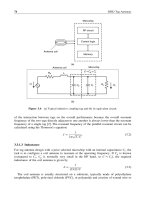
The angular patterns (Figure 6.28) present reasonable omnidirectional behaviour of the
sensor antenna with maximum variation of 8–10 dB for free space cases (off-body). Following
the set-up described above, path loss analysis of the radio channel between the Tx sensor
and a receiving antenna for cases where the sensor placed is in free space and on the body
in the anechoic chamber and in the indoor environment is performed. Figure 6.29 shows the
6.4 Case Study 225
Figure 6.27 Philips test module sensor placed on the body for radio channel characterization
measurement.
-30
-20

-10
0 dB
30
210
60
240
90
270
120
300
150
330
180
0
Tx Horizontal Free Space
Tx Vertical Free Space
Tx Onbody
-30
-20
-10
0 dB
30
210
60
240
90
270
120
300
150

330
180
0
Tx Horizontal Free Space
Tx Vertical Free Space
Tx Onbody
Figure 6.28 Received power pattern when Tx (sensor) is placed 88 cm from a receiving patch antenna
for horizontal and vertical sensor placements.
226 Antennas for Wearable Devices
-2 -1 0 1 2 3 4
55
60
65
70
y = 1.3*x + 59
OnBody-Standing
Fitted Line
OnBody-NLOS
OnBody-Sitting
OffBody-Hor
OffBody-Ver
)Bd( ssoL htaP
10*log(d/d
0
)
55
y = 1.3*x + 59
OnBody-Standing
Fitted Line
OnBody-NLOS

OnBody-Sitting
OffBody-Hor
OffBody-Ver

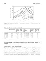
Figure 6.29 Indoor measured path loss when sensor is placed off and on body with modelled path
loss using the least fit square technique.
path loss measured in the indoor environment. As predicted, the exponent is lower than that
of free space with a value of 1.3 when the sensor is placed on the body due to multipath
components from the different scatterers. For similar distances the loss is higher for non-
line-of-sight (NLOS) cases. The directivity of the antenna increases when it is placed on the
body, as discussed earlier, due to high losses at 2.4 GHz of the human tissue which leads to
greater received power for the same distances as applied in the standalone sensor case.
6.5 Summary
Wireless body area networks have been made possible by the emergence of small and
lightweight wireless systems such as Bluetooth
™
enabled devices and PDAs. Antennas are
an essential part of any WBAN system and, due to varying requirements and constraints,
careful consideration of their design and deployment is needed.
This chapter introduced wireless body area networks and their progression from WLAN
and WPAN to satisfy the demand for more personal systems. The main requirements and
features of wearable antennas were presented with regard to design and implementation
issues. A review of the latest developments in body-worn antennas and devices provided a
clearer picture of the current state of the art and the potential areas for additional investigations
and applications. As an inseparable part of the whole communication system, specifically
in WBAN, the influence of different antenna parameters and types on the radio propagation
channel is of great significance, especially when designing antennas for wearable personal
technologies.
References 227
A case study on a compact wearable antenna used in sensors designed for healthcare

applications was presented. Antenna performance was investigated numerically with regard
to impedance matching, radiation patterns, gain and efficiency. The small size of the sensor
made it susceptible to variable changes caused by the human body and movements, specif-
ically radiated power, efficiency and the front–back ratio of radiated energy. The antenna
performance evaluation and radio propagation characterization provided indications of poten-
tial developments in designing optimum performance sensors. Improvements are necessary
in antenna design, matching circuitry and also sensor layout for better coverage area and
also to achieve the maximum range with respect to the transceiver module.
References
[1] />[2] E. Jovanov, A. Milenkovic, C. Otto and P.C de Groen, A wireless body area network of intelligent motion
sensors for computer assisted physical rehabilitation. Journal of NeuroEngineering and Rehabilitation, March
2005.
[3] S. Park and S. Jayaraman, Enhancing the quality of life through wearable technology. IEEE Engineering in
Medicine and Biology Magazine, 22 (2003), 41–48.
[4] J. Bernard, P. Nagel, J. Hupp, W. Strauss, and T. von der Grün, BAN – Body area network for wearable
computing. Paper presented at 9th Wireless World Research Forum Meeting, Zurich, July 2003.
[5] S. Matsushita, A headset-based minimized wearable computer. IEEE Intelligent Systems, 16 (2001), 28–32.
[6] P. Lukowicz, U. Anliker, J. Ward, G. Troster, E. Hirt, C. Neufelt, AMON: a wearable medical computer for
high risk patients. Proceedings of the Sixth International Symposium on Wearable Computers 2002, Seattle,
WA, October 2002, pp. 133–134.
[7] C. Kunze, U. Grossmann, W. Stork, and K. Müller-Glaser, Application of ubiquitous computing in personal
health monitoring systems. Biomedizinische Technik: 36th Annual Meeting of the German Society for Biomed-
ical Engineering, 2002, pp. 360–362.
[8] C. Balanis, Antenna Theory Analysis and Design. New York: John Wiley & Sons, Inc., 1997.
[9] /tissprop/
[10] C. Gabriel and S. Gabriel, Compilation of the dielectric properties of body tissues at RF and microwave
frequencies, 1999. />[11] Federal Communications Commission, First Report and Order, Revision of the Part 15 Commission’s Rules
Regarding Ultra-Wideband Transmission Systems, ET-Docket 98–153, April 22, 2002.
[12] D. Lamensdorf and L. Susman, Baseband-pulse-antenna techniques. IEEE Antennas and Propagation Maga-
zine, 36 (1994), 20–30.

[13] X. Qing and Z.N. Chen, Transfer functions measurement for UWB antenna. Proceedings of the IEEE
Antennas and Propagation Society International Symposium and USNC/URSI National Radio Science Meeting,
Monterey, CA, June 2004.
[14] J.S. McLean, H. Foltz and R. Sutton, Pattern descriptors for UWB antennas. IEEE Transactions on Antennas
and Propagation, 53 (2005).
[15] Internet resources, Smart textiles offer wearable solutions using Nanotechnology, URL: re2
fashion.com/news/
[16] Internet resource, Ubiquitous Communication Through Natural Human Actions, URL: tacton.
com/en/
[17] B. Sinha, Numerical modelling of absorption and scattering of EM energy radiated by cellular phones by human
arms. IEEE Region 10 International Conference on Global Connectivity in Energy, Computer, Communication
and Control, New Delhi, December 1998, Vol. 2, pp. 261–264.
[18] J. Wang, O. Fujiwara, S. Watanabe, Y. Yamanaka, Computation with a parallel FDTD system of human-body
effect on electromagnetic absorption for portable telephone. IEEE Transactions on Microwave Theory and
Techniques, 52 (2004), 53–58.
[19] H. Adel, R. Wansch and C. Schmidt, Antennas for a body area network. Proceedings of the IEEE Antennas
and Propagation Society International Symposium, Columbus, OH, June 2003, Vol. 1, pp. 471–474.
228 Antennas for Wearable Devices
[20] Body worn squad level antennas. />BodyWorn.PDF
[21] Wearable antennas: integration of antenna technologies with textiles for future warrior systems. http://www.
natick.army.mil/soldier/media/fact/individual/Antenna_Wearable.html
[22] Harris Broadband Body-Worn Dipole Antenna (30–108 MHz). />antennas-accessories/
[23] Wearable Antenna Designs LBE Integrated Shoulder Antenna (LISA). />wearable.htm
[24] P. Salonen, L. Sydänheimo, M. Keskilammi, and M. Kivikoski, A small planar inverted-F antenna for wearable
applications. Third International Symposium on Wearable Computers, 18–19 October 1999, pp. 95–100.
[25] P. Salonen, M. Keskilammi, and L. Sydänheimo, Antenna design for wearable applications. Tampere University
of Technology, Finland.
[26] P. Salonen, Y. Rahmat-Samii, H. Hurme and M. Kivikoski, Dual-band wearable textile antenna. Proceedings
of the IEEE Antennas and Propagation Society International Symposium, Monterey, CA, 20–25 June 2004,
Vol. 1, pp. 463–466.

[27] P. Salonen and L. Hurme, A novel fabric WLAN antenna for wearable applications. Proceedings of the IEEE
Antennas and Propagation Society International Symposium, Columbus, OH, 22–27 June 2003, Vol. 2, pp.
700–703.
[28] C. Cibin, P. Leuchtmann, M. Gimersky, R. Vahldieck and S. Moscibroda, A flexible wearable antenna.
Proceedings of the IEEE Antennas and Propagation Society International Symposium, Monterey, CA, 20–25
June 2004, Vol. 4, pp. 3589–3592.
[29] A. Tronquo, H. Rogier, C. Hertleer and L. Van Langenhove, Robust planar textile antenna for wireless body
LANs operating in 2.45 GHz ISM band. IEE Electronics Letters, 42 (2006), 142–143.
[30] M. Klemm, I. Locher and G. Troster, A novel circularly polarized textile antenna for wearable applications.
7th European Conference on Wireless Technology, 2004, pp. 285–288.
[31] P. Salonen, Y. Rahmat-Samii and M. Kivikoski, Wearable antennas in the vicinity of human body, Proceedings
of the IEEE Antennas and Propagation Society International Symposium, Monterey, CA, 20–25 June 2004,
Vol. 1, pp. 467–470.
[32] Z.N. Chen, A. Cai, T.S.P. See, X. Qing and M.Y.W. Chia, Small planar UWB antennas in proximity of the
human head. IEEE Transactions on Microwave Theory and Techniques, 54 (2006), 1846–1857.
[33] M. Klemm, I.Z. Kovacs, G.F. Pedersen and G. Troster, Novel small-size directional antenna for UWB
WBAN/WPAN applications. IEEE Transactions on Antennas and Propagation, 53 (2005), 3884–3896.
[34] A. Alomainy, Y. Hao, A. Owadally, C.G. Parini, Y. Nechayev, P.S. Hall and C.C. Constantinou, Statistical
analysis and performance evaluation for on-body radio propagation with microstrip patch antennas. IEEE
Transactions on Antennas and Propagation.
[35] A. Alomainy, Y. Hao, C. G. Parini and P.S. Hall, Characterisation of printed UWB antennas for on-body
communications. IEE Wideband and Multi-band Antennas and Arrays, Birmingham, UK, 7 September 2005.
[36] Y. Zhao, Y. Hao, A. Alomainy and C.G. Parini, UWB on-body radio channel modelling using ray theory
and sub-band FDTD method. IEEE Transactions on Microwave Theory and Techniques, Special Issue on
Ultra-Wideband, 54 (2006), 1827–1835.
[37] A. Alomainy, Y. Hao, X. Hu, C.G. Parini and P.S. Hall, UWB on-body radio propagation and system modelling
for wireless body-centric networks. IEE Proceedings Communications, Special Issue on Ultra Wideband
Systems, Technologies and Applications, 153 (2006).
[38] T. Zasowski, F. Althaus, M. Stager, A. Wittneben, and G. Troster, UWB for noninvasive wireless body area
networks: channel measurements and results. Proceedings of the IEEE Conference on Ultra Wideband Systems

and Technologies, Reston, VA, November 2003, pp. 285–289.
[39] J. Ryckaert, P. De Doncker, R. Meys, A. de Le Hoye and S. Donnay, Channel model for wireless communication
around human body. Electronics Letters, 40 (2004), 543–544.
[40] A. Fort, C. Desset, J. Ryckaert, P. De Doncker, L. Van Biesen and S. Donnay, Ultra wideband body area
channel model. International Conference on Communications, Seoul, May 2005.
[41] A. Fort, C. Desset, J. Ryckaert, P. De Doncker, L. Van Biesen and P. Wambacq, Characterization of the ultra
wideband body area propagation channel. International Conference on Ultra-WideBand, Zurich, September
2005.
[42] X. Qing and Z.N. Chen, Transfer functions measurement for UWB antenna. IEEE Antennas and Propagation
Society International Symposium and USNC/URSI National Radio Science Meeting, Monterey, CA, June 2004.
References 229
[43] A. Alomainy, Y. Hao, C.G. Parini and P.S. Hall, Comparison between two different antennas for UWB
on-body propagation measurements. IEEE Antennas and Wireless Propagation Letters, 4 (2005), 31–34.
[44] A. Alomainy and Y. Hao, Radio channel models for UWB body-centric networks with compact planar antenna.
Proceedings of the IEEE Antennas and Propagation Society International Symposium, Albuquerque, NM,
9–14 July 2006.
[45] P.S. Hall and Y. Hao, Antennas and Propagation for Body-Centric Wireless Networks. Boston: Artech House,
2006.
[46] Chipcon CC2420 transceiver chip, 2.4 GHz IEEE 802.15.4 / ZigBee-ready RF Transceiver, URL: http://www.
chipcon.com/files/CC2420_Data_Sheet_1_4.pdf

7
Antennas for UWB Applications
Zhi Ning Chen and Terence S.P. See
Institute for Infocomm Research, Singapore
Ultra-wideband (UWB) is one of the most promising technologies for future high-data-
rate wireless communications, high-accuracy radars, and imaging systems. Compared with
conventional broadband wireless communication systems, the UWB system operates within
an extremely wide bandwidth in the microwave band and at a very low emission limit. Due to
the system features and unique applications, antenna design is facing a variety of challenging

issues such as broadband response in terms of impedance, phase, gain, radiation patterns
as well as small or compact size. This chapter will address the antenna design issues in
UWB systems. First, the UWB technology and regulatory environment is briefly introduced;
general information on UWB systems is provided. Next, the challenges in UWB antenna
design are described. The special design considerations for UWB antennas are summarized.
State-of-the-art UWB antennas are also reviewed. UWB antennas for fixed and mobile
devices are presented. Finally, a new concept for the design of a small UWB antenna with
reduced ground-plane effect is introduced and applied to a practical scenario where a small
printed UWB antenna is installed on a laptop computer.
7.1 UWB Wireless Systems
The term ‘ultra-wideband’ (UWB) usually refers to a technology for the transmission of
information spread over an extremely large operating bandwidth where the electronic systems
should be able to coexist with other electronic users. UWB technology has been around for
decades. Its original applications were mostly in military systems. However, the first Report
and Order by the Federal Communications Commission (FCC) authorizing the unlicensed
use of UWB on February 14, 2002, gave a huge boost to the research and development
efforts of both industry and academia [1]. The intention is to provide an efficient use of
scarce frequency spectra, while enabling short-range but high-data-rate wireless personal
area network (WPAN) and long-range but low-data-rate wireless connectivity applications,
as well as radar and imaging systems, as shown in Table 7.1.
Antennas for Portable Devices Zhi Ning Chen
© 2007 John Wiley & Sons, Ltd
232 Antennas for UWB Applications
Table 7.1 Frequency ranges for various types of UWB systems under
−41.3 dBm EIRP emission limits [1]
Applications Frequency range (GHz)
Indoor communication systems 3.1–10.6
Ground-penetrating radar, wall imaging 3.1–10.6
Through-wall imaging systems 1.61–10.6
Surveillance systems 1.99–10.6

Medical imaging systems 3.1–10.6
Vehicular radar systems 22–29
According to Part 15.503 of the FCC rules, the following technical terms can be defined
for UWB operation.
•
UWB bandwidth is the frequency range bounded by the points that are 10 dB below the
highest power emission with the upper edge f
h
and the lower edge f
l
. Thus, the center
frequency f
c
of the UWB bandwidth is designated as
f
c
=
f
h
+f
1
2
 (7.1)
Accordingly, the fractional bandwidth BW is defined as
BW = 2
f
h
−f
1
f

h
+f
1
× 100% (7.2)
=
f
h
−f
1
f
c
× 100%
•
A UWB transmitter is an intentional radiator that, at any point in time, has a fractional
bandwidth BW of at least 20 % or has a UWB bandwidth of at least 500 MHz, regardless
of the fractional bandwidth.
•
Effective isotropically radiated power (EIRP) represents the total effective transmit power
of the radio, i.e. the product of the power supplied to the antenna with possible losses due
to an RF cable and the antenna gain in a given direction relative to an isotropic antenna.
The EIRP, in terms of dBm, can be converted to the field strength, in dBV/m at 3 meters,
by adding 95.2. With regard to this part of the rules, EIRP refers to the highest signal
strength measured in any direction and at any frequency from the UWB device, as tested
in accordance with the procedures specified in Part 15.31(a) and 15.523 of the FCC rules.
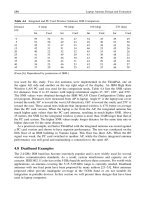
The emission limit masks are regulated by the regulators such as the FCC as shown
in Figure 7.1. The emission power limits are lower than the noise floor in order to avoid
possible interference between UWB devices and existing electronic systems. The masks
vary in different regions, but the maximum emission levels are always kept lower than
−41.3 dBm/MHz.
Furthermore, according to the FCC, any transmitting system which emits signals having a

bandwidth greater than 500 MHz or 20 % fractional bandwidth can gain access to the UWB
7.2 Challenges in UWB Antenna Design 233
Figure 7.1 Emission limit masks for indoor and outdoor UWB applications.
spectrum. Thus, both the traditional pulse-based systems transmitting each pulse which entirely
or partially occupies the UWB bandwidth, and the carrier systems based on, for instance, the
orthogonal frequency-division multiplexing (OFDM) method with a collection of narrowband
carriers of at least 500 MHz can utilize the UWB spectrum under the FCC’s rules.
The extremely large spectrum provides the room to use extremely short pulses in the order
of picoseconds. Thus, the pulse repetition or data rates can be low or very high, typically
several gigapulses per second. The pulse rates are dependent on the applications. For instance,
radar and imaging systems prefer low pulse rates in the range of a few megapulses per
second. Pulsed or OFDM communication systems tend to use high data rates, typically in
the range of 1–2 gigapulses per second, to achieve gigabit-per-second wireless connection,
although the communication range may be very short, typically a few meters. However,
the use of high data rates can enable the efficient transfer of data from digital camcorders,
wireless printing of digital pictures from a camera without the need for an intervening
personal computer, as well as the transfer of files among cellphones and other handheld
devices such as personal digital audio, video players, and laptops.
7.2 Challenges in UWB Antenna Design
One of the challenges for the implementation of UWB systems is the development of a
suitable or optimal antenna. From a systems point of view, the response of the antenna should
cover the entire operating bandwidth. The response or specifications of an antenna will vary
according to system requirements. Therefore, it is important for an antenna engineer to be
familiar with the requirements of the system before designing the antenna.
Generally, in UWB antenna design, both the frequency and time-domain responses should
be taken into account. The frequency-domain response includes impedance, radiation, and
transmission. The impedance bandwidth is measured in terms of return loss or voltage
standing wave ratio (VSWR). Usually, the return loss should be less than −10 dB or
234 Antennas for UWB Applications
VSWR < 2:1. An antenna with an impedance bandwidth narrower than the operating band-

width tailors the spectrum of transmitted and received signals, acting as a bandpass filter
in the frequency domain, and reshapes the radiated or received pulses in the time domain.
The radiation performance includes radiation efficiency, radiation patterns, polarization, and
gain. The radiation efficiency is an important parameter especially for small antenna design,
where it is difficult to achieve impedance matching due to small radiation resistance and
large reactance. For a small antenna with weak radiation directivity, the radiation efficiency
is of greater practical interest than the gain. The radiation patterns show the directions where
the signals will be transmitted.
Different from narrowband and conventional broadband systems, the requirements of the
antennas are dependant on modulation schemes. So far, two modulation schemes, namely
the multiple-carrier OFDM and pulsed direct sequence code division multiple access (DS-
CDMA) have been proposed for high-data-rate wireless communications. In these schemes,
the UWB band can be occupied in different ways. Figure 7.2 illustrates the spectra of the
OFDM and pulse-based UWB systems, which are compliant with the FCC’s emission limit
masks for indoor and outdoor applications. For instance, the emission mask can be divided
into 15 sub-bands, with each band having a bandwidth of 500 MHz as shown in Figure 7.2(a).
Alternatively, the entire UWB band can be occupied by a single pulse or several pulses, as
shown in Figure 7.2(b).
In order to coexist with the devices based on IEEE 802.11a (UNII) within the operating
frequency range of 5.150-5.825 GHz, some methods have been applied in such UWB systems.
In an OFDM-based UWB system, the sub-bands falling in the UNII range, namely the fourth,
fifth and sixth lower sub-bands in Figure 7.2(a), can be suspended. In a pulse-based UWB
system, by modulating the pulses with carriers, the spectrum can be notched to solve the
possible interference problem as depicted in Figure 7.2(b). In the figure, the spectrum can
be notched at 5-6 GHz by modulating the pulses at the carrier frequencies of 4 GHz and
8.5 GHz.
Due to the different occupancy of the UWB band in the two types of UWB system
shown in Figure 7.2, the considerations for selection of the source pulses and templates,
and design of antennas are distinct, as discussed by Chen et al. [2]. Chen et al. concluded
that the response of an antenna to UWB pulses can be described in terms of its temporal

characteristics, while it may be more intuitive for antenna engineers to consider the antenna
performance in the frequency domain [2]. In the frequency domain, an ideal UWB antenna
is required to work well across the entire UWB band with acceptable radiation efficiency,
gain, return loss, radiation pattern and polarization.
In an OFDM-based system, each sub-band having a few hundred megahertz (larger than
500 MHz) can be considered as broadband. Within the sub-bands, the effect of non-linearity
of the phase shift on the reception performance can be ignored because the phase varies very
slowly with frequency. Therefore, the design of the antenna is more focused on achieving
constant frequency response in terms of the radiation efficiency, gain, return loss, radiation
patterns, and polarization over the operating band, which may fully or partially cover the
UWB bandwidth of 7.5 GHz.
For pulse-based systems, in order to prevent the distortion of the received pulses, an ideal
UWB antenna should produce radiation fields of constant magnitude and a phase shift that
varies linearly with frequency.
By way of comparison, four types of antenna are shown in Figure 7.3: a thin strip dipole
antenna operating with a narrow bandwidth (which we will refer to as antenna A); a diamond
7.2 Challenges in UWB Antenna Design 235
Figure 7.2 Spectra of OFDM and pulse-based UWB systems compliant with the FCC’s emission
limit masks for indoor and outdoor UWB applications.
236 Antennas for UWB Applications
~
3.4
25.4
20
11.2
3
y
x
~
8.5

2
2.2
x
y
(a) (b)
~
29.75
3.2
16.65
τ
= 0.8
σ
= 0.14
f
l
= 3 GHz
f
u
= 10 GHz
1.79
z
x
(c)
~
10.5
2.2
2
y
x
(d)

Figure 7.3 Four types of antennas. (a) Antenna A: thin strip dipole antenna; (b) Antenna B: diamond
dipole antenna; (c) Antenna C: log-periodic antenna; and (d) Antenna D: circular dipole antenna.
Dimensions in millimetres.
dipole antenna having a broad operating bandwidth (B); a typical log-periodic antenna with
high gain and a broad operating bandwidth (C); and a circular dipole antenna with a very
broad operating bandwidth (D). The spectral and temporal characteristics of these antennas
are compared using Zeland IE3D, an electromagnetic simulator based on the method of
7.2 Challenges in UWB Antenna Design 237
v
t
(t

), i
t
(t

)
G
t
(ω)
v
r
(t ), i
r
(t )
G
r
(ω)
Z
L

Transmit
Antenna
Receive
Antenna
i
t
(t, l )
L
t
l
i
r
(t, l )
|E
θ rad
|
θ
L
r
l
x
y
z
r
Antenna
system
S
11
(ω)
Z

0
v
t
(t ) or V
t
(ω)
Z
load
S
22
(ω) Z
0

S
21
/S
12
(ω)
v
r
(t ) or V
r
(ω)
Z
0
H (ω)
Figure 7.4 A transmit–receive antenna system.
moments. In the comparison, the transfer function can be defined using the system shown
in Figure 7.4. As mentioned in [2], it is clear that the UWB system response between the
transmit and receive antennas is frequency-dependent. The conventional Friis transmission

formula is modified as follows:
P
r

P
t

=

1 −
t

2

1 −
r

2

G
r
G
t
ˆ
t
ˆ
r

2



4r

2
 (7.3)
The relationship between the source and output signal (voltage) can be written as:
V
t
/2
2
/2= P
t
Z
0

V
2
r
/2= P
r
Z
load

(7.4)
Thus, the transfer function in (7.3) can be simplified to give
H =
V
r

V

t

=






P
r

P
t

Z
load
4Z
0





e
−j
=

H


e
−j
 =
t
 +
r
 +r/c (7.5)
where c denotes velocity of light, and 
t
 and 
r
 are the phase shift due to the transmit
and receive antennas, respectively. As a result, if the effect of the RF channel is not taken
into account, the transfer function H is determined by the characteristics of both transmit
238 Antennas for UWB Applications
and receive antennas, such as impedance matching, gain, polarization matching, the distance
between the antennas, and the orientation of the antennas. Therefore, the transfer function
H can be used to describe general antenna systems, which may be dispersive.
Furthermore, the transmit-receive antenna system can be considered as a two-port network.
The transfer function H can be measured in terms of S
21
when the source impedance
and load are matched to the antenna input and output, respectively. This implies that the
measurable parameter S
21
or H is able to integrate all the important system parameters
in terms of gain, impedance matching, polarization matching, path loss, and phase delay.
Therefore, they can be used to assess the performance of UWB antenna systems and other
antenna systems whose performance is frequency-dependent.
In the measurement of H, the orientations of the transmit and receive antennas are

shown in Figure 7.5. Identical antennas are used as transmit and receive antennas in the
test setup shown in the figure. Figure 7.5(a) shows a pair of antennas B with a separation
100 mm
x ′
y
z
~
~
x
y ′
z ′
(a)
~
~
100 mm
z
x
x ′
z ′
(b)
Figure 7.5 Orientation of antennas: (a) antenna B (antennas A and D placed in the same position);
(b) antenna C.
7.2 Challenges in UWB Antenna Design 239
of 100 mm and positioned in parallel and face-to-face. Similarly, antennas A and D are
positioned face-to-face in the same orientation with a separation of 100 mm, while a pair of
antennas C is placed tip-to-tip with a separation of 100 mm as shown in Figure 7.5(b).
Figure 7.6 demonstrates the return losses S
11
 and the magnitude of the transfer function
S

21
 for antennasA–D.Itisclear from Figure 7.6(a) that antenna A has a narrow-
band impedance and transmission response. The antenna is well matched around the center
frequency of the UWB band (7 GHz). Around 6–7 GHz, the transmission reaches its peak
and subsequently decreases gradually.
From Figure 7.6(b), it is evident that the impedance bandwidth of antenna B, for 10 dB return
loss, covers the whole UWB band very well. However, the 10 dB bandwidth for the transmission
only ranges from 2 to 6 GHz, partially covering the lower range of the UWB band.
Antenna C displays broadband characteristics for both impedance and transmission, as
shown in Figure 7.6(c). Compared with the other three antenna designs, antenna C is much
larger in size and more directional in radiation with a high system gain of −18 to −15 dB.
Antenna D shows broad impedance bandwidth covering the entire UWB band and broad
transmission coverage from 2 to 8.5 GHz within a 10 dB variation (Figure 7.6(d)).
Figure 7.6 Comparison of the return loss S
11
 and of the transfer function S
21
 for (a) antenna A;
(b) antenna B; (c) antenna C; (d) antenna D.
240 Antennas for UWB Applications
The comparison of the system gain for transmission shows that antenna C has the highest
peak gain of −15 dB, whereas antenna A has the lowest peak gain of −25 dB. Antennas B
and D have the same peak gain of −18 dB.
Due to the ultra-wide operating bandwidth of UWB systems, the phase response of the
transmission may not be linear. This feature differentiates the design considerations for
the pulse-based UWB antennas from those in narrowband systems and OFDM-based UWB
systems [2]. The non-linear phase response may severely distort the waveforms of short
pulses in the form of ringings. The phase responses of S
21
 for antennasA–Dareshown in

Figure 7.7. The non-linear phase response of antenna C over the UWB band is demonstrated
in Figure 7.7(c). The phase centers shift with frequency because the main radiation at a
frequency f
r
always occurs at the dipole with a length of around a half-wavelength at f
r
.
Therefore, the phase centers at lower operating frequencies are located around longer dipoles,
and conversely around shorter dipoles at higher operating frequencies.
Figure 7.8 shows the radiation patterns for antennasA–Dat3,5,7,and9GHz. Antennas
A, B, and D are basically dipole antennas and show typical radiation characteristics especially
at the lower operating frequencies, namely an omnidirectional radiation in the horizontal plane
Figure 7.7 Comparison of the phase response of S
21
: (a) antenna A; (b) antenna B; (c) antenna C;
and (d) antenna D.
7.2 Challenges in UWB Antenna Design 241
–10 0
–90°
90°
E
θ
, φ = 0°
E
φ
, φ = 0°
E
θ
, φ = 90°
E

φ
, φ = 90°
7 GHz
θ = 0°(10 dBi)
180°
(a)
7 GHz
(b)
–10
0
E
θ
, φ = 0°
E
φ
, φ = 0°
E
θ
, φ = 90°
E
φ
, φ = 90°
–10
0
–90°
3 GHz
θ = 0°(10 dBi)
180°
90°
–10

–90°
θ = 0°(10 dBi)
180°
90°
5 GHz
–10
0
–90°
θ = 0°(10 dBi)
180°
90°
9 GHz
0
–90°
θ = 0°(10 dBi)
180°
90°
Figure 7.8 Comparison of the radiation patterns at 3, 5, 7, and 9 GHz: (a) antenna A; (b) antenna B;
(c) antenna C; (d) antenna D.
242 Antennas for UWB Applications
(c)
7 GHz
0
0
E
θ
, φ = 0°
E
φ
, φ = 0°

E
θ
, φ = 90°
E
φ
, φ = 90°
–90°
3 GHz
θ = 0°(20 dBi)
180°
90°
–20
–20
–90°
θ = 0°(20 dBi)
180°
90°
5 GHz
–20
0
–90°
θ = 0°(20 dBi)
180°
90°
–20
9 GHz
0
–90°
θ = 0°(20 dBi)
180°

90°
7 GHz
(d)
–10
0
E
θ
, φ = 0°
E
φ
, φ = 0°
E
θ
, φ = 90°
E
φ
, φ = 90°
–10
0
–90°
3 GHz
θ = 0°(10 dBi)
180°
90°
–10
–90°
θ = 0°(10 dBi)
180°
90°
5 GHz

–10
0
–90°
θ = 0°(10 dBi)
180°
90°
9 GHz
0
–90°
θ = 0°(10 dBi)
180°
90°
Figure 7.8 (Continued).
7.2 Challenges in UWB Antenna Design 243
and inverted figure-of-eight radiation in the vertical planes. However, at higher frequencies
the radiation patterns of the broadband antennas B and D vary significantly because the
antenna size has become electrically large. In the horizontal plane, the radiation becomes
directional. The radiation patterns of antenna B have nulls in the horizontal plane at 7 and
9 GHz. This has narrowed the transmission response of antenna B to a great extent, as shown
in Figure 7.6(b) along the z-axis direction. As mentioned above, antenna C is a directional
antenna with a high and stable gain along its tip direction.
In order to examine the effects of performance of the transmit and receive antennas
on the received signals in a pulsed system, the impulse responses of the four antenna
systems are illustrated in Figure 7.9. Because antenna A has the narrowest bandwidth and
lowest gain, the pulse received has the lowest magnitude and experiences more ringing.
For antenna C, with the broadest bandwidth and highest gain but a non-linear phase
response, the received pulse has a higher magnitude but experiences the most severe distor-
tion with significant ringing. Comparing the waveforms of the pulses received by antennas
B and D with acceptable gain, it is evident that the magnitude of the received pulse
Figure 7.9 Impulse response at the load of the receive antenna: (a) antenna A; (b) antenna B; (c)

antenna C; (d) antenna D.
244 Antennas for UWB Applications
Table 7.2 Summary of antenna performance.
Antenna Impedance bandwidth System gain/bandwidth Phase response Suitable
for systems
OFDM/pulsed
A Narrow Lowest/narrowest Linear No/No
B UWB band Acceptable/narrower Linear No
a
/Yes
C UWB band Highest/widest Non-linear Yes/No
D UWB band Acceptable/acceptable Linear Yes/Yes
a
The bandwidth of the system gain is still broad and covers part of the UWB band, for example, the
lower portion of the UWB band of 3.1–5 GHz, which is widely used in high-speed/short-range mobile
devices.
of antenna D is 30 % higher than that of antenna B, and they both have less ringing than
antenna C. A summary of the performance of antennas A–D is given in Table 7.2.
The assessment of the antennas should be performed from an overall systems point of
view and not just that of an antenna element. As such, there are three parameters, namely the
fidelity, system gain, and EIRP bandwidth, which can be used to analyze the performance
of the antenna in transmit – receive antenna systems. In order to illustrate the concept of
the three parameters more clearly, we will take the circular dipole antenna (D) as an example.
In this study, the sine modulated Gaussian pulse has been chosen as the source pulse.
The monocycle pulses are modulated at frequencies of f
s
= 4 7, and 8.5 GHz, which corre-
sponds closely to the center frequency of the lower UWB band (3.1–5 GHz), the entire UWB
band (3.1–10.6 GHz), and the upper UWB band (6–10.6 GHz), respectively. With optimiza-
tion, the pulse parameter  for the template pulse as well as the modulation frequency

of the template pulse can be obtained for a fixed modulation frequency of the source
pulse f
s
.
First, the fidelity parameter is used to measure the performance of the pulsed UWB
systems in [2, 3]. The fidelity of the pulses of an antenna system can be calculated to assess
the quality of a received pulse and select a proper detection template. The fidelity can be
defined as
F =max



−
Lp
source
tp
output
t −dt (7.6)
where the source pulse p
source
t and output pulse p
output
t are normalized by their respective
energies. The fidelity F is the maximum value of the integral by varying time delay  with
respect to the source pulse. The linear operator L· operates on the input pulse p
source
t.
Evidently, the template at the output of a receiving antenna may most probably be Lp
source
t

and not p
source
t in order to achieve maximum fidelity.
Figure 7.10 plots the fidelity obtained for different modulation frequencies of the source
pulse f
s
. With a proper selection of the source pulse parameter  and the modulation
frequency f
t
for the template pulse, maximum fidelity can be achieved. It should be noted
that in this case the antenna has a broad operating bandwidth so that the distortion of the
waveforms of the received pulses is slight. As a result, the frequency f
t
is very close to the
7.2 Challenges in UWB Antenna Design 245
2
0.0
0.2
0.4
0.6
0.8
1.0
Fidelity
f
t
, GHz
f
s
= 4 GHz, σ = 366 ps
f

s
= 7 GHz, σ = 99 ps
f
s
= 8.5 GHz, σ = 78 ps
1211109876543
Figure 7.10 Comparison of fidelity against template pulse.
frequency f
s
. Otherwise, the difference between the frequencies f
s
and f
t
will be large due
to the severe distortion of the waveforms of the received pulses [2].
Also, the source pulse has been properly chosen such that the radiated spectra are able to
comply with the FCC’s emission limits as shown in Figure 7.11. Therefore, in the selection and
optimization of the source and template pulses, the compliance with the FCC’s emission limit
masks and maximum fidelity are two key factors which should be taken into consideration.
The system gain parameter can be used to evaluate the efficiency of a transmit-receive
antenna system and can be calculated from
G
sys
= 16r
2
R
0


0

V
2
r
t   



dt
R
load


0
V
2
t
tdt
(7.7)
Figure 7.11 Spectra of radiated pulses for different source pulses.
246 Antennas for UWB Applications
where V
t
and V
r
are the source and output voltages, respectively; R
0
and R
load
are the source
and load resistances, respectively; ,  indicate the elevation and azimuth angles of the

transmitting antenna; 

, 

denote the elevation and azimuth angles of the receiving antenna;
and r is the distance between the antennas. Clearly, G
sys
not only depends on the impedance
matching of the antennas but also on their directivities, which are angle-dependent.
The EIRP bandwidth is defined as the bandwidth within which the EIRP of the radiated
spectrum is 10 dB below the maximum. This is the parameter used to measure the efficiency
of occupation of the operating bandwidth. In this case, since the radiated spectrum is to be
within the indoor emission limits from 3.1 to 10.6 GHz, the EIRP bandwidth will not exceed
7.5 GHz.
Figure 7.12 plots the variation of the system gain and EIRP bandwidth against the source
pulse parameter . The lower bound for  is set at 366, 99, and 78 ps for f
s
= 47, and
8.5 GHz, respectively. It should be noted that any value less than the lower bound will result
in the failure of the radiated spectrum to conform to the FCC’s emission limits. Due to the
variation of the antenna gain along the z-axis as shown in Figure 7.6(d), the optimum system
gain varies from −33 dB
∗
m
2
(for f
s
= 85 GHz) to −28.5 dB
∗
m

2
(for f
s
= 4 GHz).
Figure 7.13 plots the variation of the fidelity against different  when the template is fixed.
In order to achieve a broad EIRP bandwidth performance,  should be chosen such that
good fidelity, high system gain, and broad EIRP bandwidth performance can be obtained.
From Figure 7.13, it is evident that the fidelity can exceed 0.8 around the optimal .
In conclusion, the UWB antenna design plays a unique role in UWB wireless communi-
cation systems. UWB systems based on distinct modulation schemes have different require-
ments in antenna design. In an OFDM-based UWB system, the requirements are almost
the same as those in a broadband system but with an extremely broad bandwidth which
usually varies from 50 % (for the lower UWB band of 3.1–5 GHz) to 100 % (for the entire
UWB band of 3.1–10.6 GHz). Special attention must be given to pulse-based UWB systems,
where a UWB antenna functions as a bandpass filter and reshapes the spectra of the radi-
ated/received pulses. In order to avoid undesirable distortions of the radiated and received
pulses, the critical requirements in antenna design include, as far as the electrical parameters
are concerned,
0
–40
–38
–36
–34
–32
–30
–28
1
2
3
4

5
6
G
sys
G
sys
, dB m
2
EIRP Bandwidth, GHz
40035030025020015010050
f
s
= 8.5 GHz
f
s
= 4 GHz
f
s
= 7 GHz
f
s
= 8.5 GHz
f
s
= 4 GHz
f
s
= 7 GHz
EIRP BW
σ

Figure 7.12 System gain and EIRP bandwidth vs. .
7.3 State-of-the-Art Solutions 247
0.2
0.4
0.6
0.8
1.0
0 40035030025020015010050
Fidelity
f
s
= 8.5 GHz
f
s
= 4 GHz
f
s
= 7 GHz
σ
Figure 7.13 Fidelity vs. .
•
ultra-wide impedance bandwidth covering the bandwidth where most of the energy of the
source pulse is concentrated;
•
steady directional or omnidirectional radiation patterns;
•
constant gain;
•
constant group delay or linear phase;
•

constant polarization; and
•
high radiation efficiency.
All of the electrical performance should be achieved over the entire operating band. The
mechanical requirements in antenna design – small size, embeddability, low profile and low
cost – stem from the applications directly because the most promising application of UWB
technology is in short-range wireless connections between mobile or handheld consumer
devices. Therefore, the size and cost issues have become critical.
In particular, OFDM-based multiband UWB systems require flat impedance and gain
response, which can cover the entire operating bandwidth. Pulse-based UWB systems require
linear phase, impedance, and gain response which can entirely cover the operating bandwidth
or partially cover the bandwidth where the majority of the pulse energy is distributed.
7.3 State-of-the-Art Solutions
7.3.1 Frequency-Independent Designs
The UWB antennas under discussion can actually be considered as frequency-independent
with an extremely broad frequency response, typically 50–100 %. For example, transverse
electromagnetic (TEM) horns feature very broad well-matched bandwidths and have been
widely studied and applied [4–6]. TEM horn antennas in their basic forms are illustrated in
Figure 7.14. A pair of triangular metal flares forms a TEM horn antenna and a feed excites
the end of the horn, as shown in Figure 7.14(a). To enhance the gain of the horn antenna,
248 Antennas for UWB Applications
Figure 7.14 TEM horn antennas in their basic forms.
a lens is used to cover the aperture of the horn, as shown in Figure 7.14(b). The antenna
radiates linearly polarized TEM waves.
Theoretically, frequency-independent antennas, which have a constant performance at
all frequencies, can also be applied to broadband antenna design. The self-complementary
log-periodic structures, such as planar log-periodic slot antennas, bidirectional log-periodic
antennas, log-periodic dipole arrays, two-or four-arm log-spiral antennas, and conical log-
spiral antennas, are a typical design [7]. The geometry of a balanced conical log-spiral
antenna is shown in Figures 7.15(a) and 7.15(b). A planar two-arm spiral antenna is shown in

Figure 7.15(c). However, for log-periodic antennas, the frequency-dependent phase centers
severely distort the waveforms of radiated pulses [8]. They radiate circularly polarized wave
at the boresight. Spiral antennas can be completely specified by angles, and they feature
constant impedance and radiation pattern performance with frequency. In practice, spiral
antennas have a finite size so the frequency-independent behavior is only exhibited over
a certain frequency range which is determined by its inner and outer radius. The planar
spiral antenna usually requires a backed cavity which is typically lossy to improve the low-
frequency impedance behavior and axial ratio by reducing the reflections from the end of the
spiral arm. The lossy cavity also absorbs the back radiation from the spiral to enhance pattern
bandwidth and achieve unidirectional, radiation usually at the boresight with an undesirable
reduction in gain. Alternatively, the spiral antennas backed by conducting cavities have been
widely used in applications which require the radiation to be directional.
Biconical antennas, constructed by Sir Oliver Lodge in 1897, are the earliest antennas used
in wireless systems, as mentioned by John D. Kraus [9]. They have relatively stable phase
centers with broad impedance bandwidths due to the excitation of TEM modes. Many diverse
variations of biconical antennas, such as finite biconical antennas, discone antennas, single-
cone with resistive loadings have since been constructed and optimized for broad impedance
bandwidth [10–12]. Figure 7.16 shows a typical biconical antenna and its variations.
Cylindrical antennas with resistive loading also feature broadband impedance characteris-
tics by forming traveling waves along the dipole arms [13–15].
7.3.2 Planar Broadband Designs
However, the antennas mentioned in Section 7.3.1 are seldom used in portable/mobile
devices due to size and cost constraints. Antennas with bulky size are usually employed