An Experimental Approach to CDMA and Interference Mitigation phần 3 pdf
Bạn đang xem bản rút gọn của tài liệu. Xem và tải ngay bản đầy đủ của tài liệu tại đây (425.65 KB, 29 trang )
2. Basics of CDMA for Wireless Communications 39
From the considerations made above, it is evident that the most peculiar
and crucial function which the DS/SS receiver has to cope with is timing re-
covery. The basic difference between the function of symbol timing recovery
in a conventional modem for narrowband signals and code alignment in a
wideband SS receiver lies in a fundamental difference in the statistical prop-
erties of the data bearing signal. In narrowband modulation the data signal
bears an intrinsic statistical regularity on a symbol interval
s
T that is, prop-
erly speaking, it is
cyclostationary with period
s
T
. Clock recovery is to be
carried out with an accuracy of some hundredths of a
s
T , and is not particu-
larly troublesome. Owing to the presence of the spreading code, the DS/SS
signal is cyclostationary with period
c
LT
(in a short code arrangement), but
the receiver has to derive a timing estimate with an accuracy comparable to
a
tenth of the chip interval
c
T to perform correlation and avoid Inter-Chip In-
terference
(ICI).
10
-6
10
-5
10
-4
10
-3
10
-2
10
-1
12108642
E
b
/
N
0
(dB)
BER(9.6 dB)=10
-5
BER(6.8 dB)=10
-3
Figure 2-9. BER of a matched-filter receiver for BPSK / QPSK transmission
over the Gaussian channel.
This simple discussion suggests that timing estimation becomes more and
more involved as
L gets large (long codes). Unfortunately, in practical
applications of DS/SS transmissions we always have 1
L even for short
40 Chapter 2
codes (typically
31L t
), so that the problem of signal timing recovery with
a sufficient accuracy is much more challenging for wideband DS/SS signals
than for narrowband modulation, and is usually split in the two phases of
coarse acquisition and fine tracking. The first is activated during receiver
startup, when the DS/SS demodulator has to find out whether the intended
user is transmitting, and, in the case in which he/she actually is, coarsely es-
timate the signal delay to initiate fine chip time tracking and data detection.
Code tracking is started upon completion of the acquisition phase and aims
at locating the optimum sampling instant of the chip rate signal to provide
ICI-free samples (such as (2.59)) to the subsequent digital signal processing
functions.
M
c
m
Chip Pulse
Matched Filter
g (t)
R
6
1
M
r(t)
~
y(t)
~
mT
c
y
m
~
z
k
~
d
k
~
^
Figure 2-10. Baseband equivalent of a DS/SS receiver.
After examining the main functions for signal detection, we present some
introductory considerations about the practical implementation of a DS/SS
receiver. In this respect Figure 2-11 shows a scheme of a DS/SS receiver
highlighting also the different signal synchronization functions (carrier fre-
quency/phase and timing) which often represent the real crux of good mo-
dem design. We have denoted by
ˆ
f
' ,
ˆ
T
, and
ˆ
W
the estimates of the carrier
frequency offset, phase offset, and chip timing error, respectively, relevant to
the useful signal. As already discussed (see Figure 2-8), the baseband I/Q
components of
()rt are derived via a baseband I/Q converter as the one in
Figure 2-3. Such a converter is usually implemented at IF in double conver-
sion receivers or directly at RF in low cost, low power receivers (this is the
case, for instance, for mobile phones).
The basic architecture of Figure 2-11 can be entirely implemented via
DSP components by performing Analog to Digital Conversion (ADC) as
early as possible, at times directly on the IF (intermediate frequency) signal
provided at the output of the RF to IF front end conversion stage in the re-
ceiver. In so doing, the baseband received signal
()rt
in Figure 2-11 is actu-
ally a sampled digital signal, carrier recovery and chip matched filtering are
digital, and the ‘sampler’ is just a decimator/interpolator that changes the
clock rate of the digital signal. The ADC conversion rate of
()rt
is, in fact,
invariably faster than the chip rate to perform chip matched filtering with no
2. Basics of CDMA for Wireless Communications 41
aliasing problems. We shall say more about the digital architecture of the
DS/SS receiver in Chapter 3 when dealing specifically with the MUSIC de-
modulator.
M
Chip Pulse
Matched Filter
g (t)
R
6
1
M
r(t)
~
y(t)
~
y
m
~
z
k
~
d
k
~
^
Carrier
Recovery
c
m
Code-Delay
Recovery
Local Code
Replica
mT + W
c
^
exp{-j2S'ft+T}
^^
Figure 2-11. Architecture of a receiver for DS/SS signals, including synchronization units.
3. CODE DIVISION MULTIPLEXING AND
MULTIPLE ACCESS
In the DS/SS schemes discussed above the data stream generated by an
information source is transmitted over a wide frequency spectrum using one
(or two) spreading code(s). Starting from this consideration we can devise an
access system allowing
multiple users to share a common channel transmit-
ting their data in DS/SS format. This can be achieved by assigning each user
a different spreading code and allowing all the signals
simultaneously access,
in DS/SS mode, the
same frequency spectrum. All the user signals are there-
fore transmitted at the
same time and over the same frequency band, but they
can nevertheless be identified thanks to the particular spreading code used,
which is different from one user to another (the so called
signature code).
The users are separated in the
code domain, instead of time or frequency
domain, as in conventional
Time or Frequency Division Multiple Access, re-
spectively (TDMA, FDMA). Such a multiple access technique, based on
DS/SS transmission, is therefore called
Code Division Multiple Access
(CDMA) and the spreading sequence identifying each user is also referred to
as
signature. The N user signals in DS/SS format can be obtained from a set
of
N tributary channels made available to a single transmitting unit which
performs spectrum spreading of each of them, followed by Code Division
Multiplexing (CDM). Alternatively, the DS/SS signals can be originated by
N spatially separated terminals, and in this latter case code division multi-
plexing occurs at the receiver antenna.
Let us focus our attention on the detection of a DS/SS signal in the case
of a
multiuser CDMA system in which N users are concurrently active. For
the sake of simplicity, we refer once again to the simplified signal model
42 Chapter 2
(2.30). We will start considering the case a CDMA multiuser communication
in which all of the spreading sequences of the different users are
synchro-
nous
, i.e., the start epoch is exactly the same for each code. We will refer to
this arrangement as
Synchronous CDMA (S-CDMA). This is the case of a
CDMA signal originated from a single transmitter, i.e., from a base station
(or satellite) to a group of mobile receivers. We will therefore address such a
scenario as
single-cell. The received signal, after baseband conversion and
under the hypothesis of perfect carrier recovery, can be written as
^`
1
M
L
N
iii
Tc
kk
ik
rt A d c g t kT wt
f
f
¦¦
, (2.70)
with the same definitions as in the single-user case described by (2.49),
where for each user’s channel we have defined the amplitude coefficient (see
(2.11))
2
2
i
i
s
d
APA
. (2.71)
Notice that, in order to take the multiple users accessing the RF spectrum
into account we have introduced the superscript
()i
which identifies the am-
plitude, data, and code chips of the generic
i
th user. The generation of the
aggregate code division multiplexed signal (2.70) is conceptually depicted in
Figure 2-12
Assuming now, without loss of generality, that the receiver intends to de-
tect the data transmitted by user 1, we can re-write (2.70) as
^`
111
M
L
Tc
kk
k
rt A d c g t kT
f
f
¦
^`
2
M
L
N
iii
Tc
kk
ik
AdcgtkTwt
f
f
¦¦
, (2.72)
where the first term at the right hand side is the useful signal to be detected,
while the second one, denoted in a more compact form as
^`
2
ML
N
iii
Tc
kk
ik
bt A d c g t kT
f
f
¦¦
(2.73)
is an additional component owed to multiple access. In a conventional corre-
lation receiver, the received signal (2.72), is passed through the chip
matched filter and sampled at chip rate yielding the samples
m
y
(see (2.59))
2. Basics of CDMA for Wireless Communications 43
^`
^`
11 1
2
MM
LL
N
ii i
mm
mm mm
i
yAd c Ad c n
¦
^`
11 1
ML
mm
mm
Ad c b n
, (2.74)
where
()
mm
bbt
is given by
^`
,,
2
j
M
L
N
ii i
mIm Qm
mm
i
bb b Ad c
¦
. (2.75)
DS/SS-BPSK
Modulator #1
DS/SS-BPSK
Modulator #2
DS/SS-BPSK
Modulator #N
…
w(t)
r(t)
DS/SS
Modulator #1
A
…
r(t)
DS/SS
Modulator #2
DS/SS
Modulator #N
~
~
c
(1)
c
(2)
c
(N)
d
(1)
d
(2)
d
(N)
(1)
A
(2)
A
(N)
Figure 2-12. Generation of a multiuser S-CDMA signal.
The I/Q components
,
I
m
b and
,Qm
b in (2.75) are independent, identically
distributed, zero mean random variables whose variance is
^
`
22 2
,
E
IQ
bb Im
bV V
. (2.76)
The sampled signal (2.74) undergoes correlation (despreading / accumu-
lation) with the signature code of user 1 as follows
1
11
1
L
kM M
km
m
mkM
zyc
M
¦
. (2.77)
After some algebra we find (see (2.61)(2.64))
44 Chapter 2
11
1
111
L
L
kM M
k
k
mm
mkM
Ad
zcc
M
¦
1
1
2
LL
ii
NkMM
i
k
k
mm
imkM
Ad
cc
M
Q
¦¦
(2.78)
and
11 1
111
2
i
N
ii
kk k k
cc cc
i
zAd k Ad k
F F Q
¦
, (2.79)
where we have defined the following partial auto- and cross-correlations
11
1
11
1
1
LL
kM M
mm
cc
mkM
kcc
M
F
¦
, (2.80)
1
1
1
1
i
L
L
kM M
i
mm
cc
mkM
kcc
M
F
¦
. (2.81)
The decision strobe is eventually passed to the final detector which re-
generates the transmitted digital data stream of the user 1 (the desired, ‘sing-
ing’ user). From (2.79) it is apparent that the decision strobe
(1)
k
z
is com-
posed of three terms: i) the useful datum (first term); ii) Gaussian noise
(third term); and iii) an additional term arising form the concurrent presence
of multiple users and called
Multiple Access Interference (MAI). In particu-
lar, the MAI term can be expressed as
1
,,
2
j
i
N
ii
kIk Qk k
cc
i
Ad k
E E E F
¦
, (2.82)
or equivalently, according to definition (2.75), as
1
1
,,
1
j
L
kM M
kIk Qk m
m
mkM
bc
M
E E E
¦
(2.83)
The I/Q components
,
I
k
E and
,Qk
E are independent, identically distrib-
uted, zero mean random variables whose variance can be put in a form simi-
lar to (2.63)
2. Basics of CDMA for Wireless Communications 45
^
`
22 2
,0
E/
IQ
I
ms
I
T
EE
V V E (2.84)
where we have introduced an equivalent PSD
0
I of the MAI term, as-
suming implicitly that it can be considered
flat (white) over the whole signal
spectrum. Now re-cast (2.79) into the form
111
kkkk
zAd EQ
. (2.85)
Under certain hypotheses which we will discuss in a little while, the MAI
contribution can be modeled as an additional (white) Gaussian noise
(independent of
k
Q
). Therefore the BER performance of the DS/SS signal
can be analytically derived simply by assuming an equivalent noise term
kkk
c
Q EQ
with a total, equivalent PSD given by
000
NNI
c
, (2.86)
and the decision strobe becomes equivalent to that in (2.67), which refers to
a pure AWGN channel
111
kkk
zAd
c
Q
. (2.87)
Consequently the BER for QPSK modulation in the presence of Gaussian
MAI, can be obtained by a simple modification of expression (2.68)
000
22
bb
EE
Pe
NNI
§·§ ·
¨¸¨ ¸
¨¸¨ ¸
c
©¹© ¹
. (2.88)
If very long pseudo-random (i.e., noise-like) spreading sequences are
used then the chips
()
||
L
i
m
c of each user code can be approximately modeled as
independent random variables belonging to the alphabet
{-1,+1}. Also, the
chips of different users can be modeled as uncorrelated random variables. It
follows that if
1N
and if all of the signal powers are (almost) equal (i.e.,
i
s
s
P
P , i ), then the power of the MAI is
MAI
(1)
s
P
NP
and by virtue of
the central limit theorem, we can model the MAI components
,
I
k
E and
,Qk
E
at the detector input as independent identically distributed zero mean Gaus-
sian random variables with variance (see (2.76) and (2.83))
22
0MAI
1
(1 / )
IQ
s
c
sc
NP
IP T
TMT M
EE
V V
. (2.89)
46 Chapter 2
This situation is actually experienced, for instance, in a CDMA system
with accurate power control, so that all the users signals are received at (al-
most) the same power level. Under this hypothesis the PSD of the MAI is
0
11
11
s
s
sc c b
p
NP N
I
TNPTNEE
MG
, (2.90)
where
csc
E
PT
represents the average energy at RF per chip, and according
to (2.40) we have set
/
cbp
E
EG . The BER (2.88) becomes then
0
2
Q
1
b
c
E
Pe
NNE
§·
¨¸
¨¸
©¹
(2.91)
and with some manipulations we obtain for QPSK
0
0
1
2
Q
1
2
1
b
b
E
Pe
N
E
N
N
M
§·
¨¸
¨¸
¨¸
¨¸
¨¸
©¹
. (2.92)
From the expressions above it turns out that the MAI degrades the BER
performance. In particular, the degradation increases with the number of in-
terfering channels and decreases for large processing gains. Notice also that,
in the particular case
1N (2.92) collapses to the conventional BER ex-
pression relevant to (narrowband) QPSK modulation over AWGN channel
and matched filter detection.
However, we must remark that in the more general case of CDMA
transmissions with MAI (
1N ! ) (2.92) is accurate only under certain condi-
tions. In particular, the assumption of uncorrelated binary random variables
for the code chips is valid only when the signature codes are ‘long’ in the
sense of Section 2. As is apparent from (2.82), the amount of MAI is in real-
ity determined by the cross-correlation properties between the useful signal
and the interferers. Therefore, in order to derive a more accurate analytical
expression for the BER the particular type of spreading codes and the rele-
vant correlation properties must be accounted for. In order to simplify the
analytical description, from now on we shall focus on the case of short
spreading codes, i.e.,
M
nL . Recalling (2.42), the cross-correlation
(2.81) is now
2. Basics of CDMA for Wireless Communications 47
1 1
11
11
11
i i
LL LL
knL nL knL L
ii
mm mm
cc cc
mknL mknL
kccnccR
nL nL
F
¦¦
. (2.93)
The variance of the I/Q components of the MAI samples
m
E
must be re-
written by resorting to (2.82), yielding
1
22 2
0
2
i
IQ i
N
s
cc
i
s
I
PR
T
EE
V V
¦
, (2.94)
and the PSD of the MAI contribution to the total noise in (2.86) becomes
1
2
0
2
i
i
N
ss
cc
i
IT PR
¦
. (2.95)
In the case of equi-powered users we obtain
11
22
0
22
ii
NN
ss s
cc cc
ii
IPT R E R
¦¦
, (2.96)
where
s
ss
E
PT represents the average energy at RF per modulation symbol.
Since, for QPSK,
/2
sb
RR
, we have
2
s
b
E
E
and therefore
1
2
0
2
2
i
N
b
cc
i
IER
¦
(2.97)
By retaining the assumption of a Gaussian distribution of the MAI, which
holds true in the case of large spreading factors and large number of users,
the BER is now
1
2
0
2
0
1
2
Q
2
1
i
b
N
b
cc
i
E
Pe
E
N
R
N
§·
¨¸
¨¸
¨¸
¨¸
¨¸
©¹
¦
. (2.98)
From the expression above we can conclude that in order to limit the
detrimental effect of MAI on BER performance the spreading sequences
must be chosen so as to exhibit the lowest possible cross-correlation level. In
the case of maximal length sequences with 1
L , the cross-correlation is
well approximated by [Sar80]
48 Chapter 2
1
1/
i
cc
R
L# (2.99)
thus, recalling that
M
nL
, we obtain
0
0
1
2
Q
1
2
1
b
b
E
Pe
n
N
E
N
M
N
§·
¨¸
¨¸
¨¸
¨¸
¨¸
©¹
, (2.100)
which for
1n coincides with the BER expression (2.92) previously de-
rived for the white Gaussian MAI model. Actually (2.99) represents the
RMS value of the cross-correlation between two
L
-period maximal length
sequences taken over all the possible relative phase shifts. However, it is
found that, in spite of their many appealing features,
m-sequences are not
convenient for CDMA. First, for a given
m there exists only a limited num-
ber of sequences available for user identification in a CDMA system
[Din98]. Also, the cross-correlation properties of
m-sequences are not opti-
mal, so they result in significant levels of MAI.
The MAI term
k
E
in (2.85) can be canceled by using orthogonal codes
such as
() ( )
0
i
j
cc
R (ijz ). A popular set of orthogonal spreading codes is
represented by the
Walsh–Hadamard (WH) sequences [Ahm75], [Din98]
which have period
2
m
L and are obtained taking the rows (or the columns)
of the
LLu matrix
m
H recursively defined as follows
11
1
11
11
,
11
mm
m
mm
ªº
ªº
«»
«»
¬¼
¬¼
HH
HH
HH
(2.101)
where
m
H
means the complement (i.e., the sign inversion) of each element
of the matrix
m
H . From (2.101) it is apparent that for a given period
L
the
WH set is composed of
L
sequences. Thanks to orthogonality the BER per-
formance for an
Orthogonal CDMA (O-CDMA) system is obtained by re-
moving the MAI contribution in (2.98), which gives the conventional ex-
pression for narrowband BPSK/QPSK modulation (2.68).
Despite such an appealing feature, it must be noticed that the WH se-
quences exhibit very poor off zero auto- and cross-correlation properties
making difficult initial code acquisition and user recognition by the receiver.
For this reason, in practical applications
pure orthogonal codes such as the
WH sequences must be used overlaid by a PN sequence [Fon96], [Din98].
According to this approach the resulting
composite code is therefore the su-
perposition
of two codes, i.e., an orthogonal WH code
()
WH
{ }{1}
i
k
c r for
2. Basics of CDMA for Wireless Communications 49
user identification (the so called
traffic or channelization code) plus an over-
lay
PN sequence
PN
{}{1}
k
c r , common to all the users within the same
cell (or satellite beam), as follows
PN
WH
ii
kk k
cc c
'
. (2.102)
The cell- (or beam-) unique overlay code yields a twofold benefit: first, it
represents a sort of cell (or beam) identifier and second, it performs a ‘ran-
domization’ of the user signature that is helpful in reducing unwanted off
zero auto- and cross-correlation peaks. For this reason the overlay code is
also called
scrambling code. It is immediate to observe also that orthogonal-
ity between any pair of composite sequences is preserved, i.e.,
() ( )
0
i
j
cc
R
( ijz ) still holds true. Finally, notice that if we want to obtain a composite
code having exactly the same period
2
m
L as the original WH sequence we
must select an overlay maximal length sequence having period 2 1
m
, and
properly extend it by inserting a ‘+1’ chip into its longest run. Such a modi-
fied sequence is called
Extended PN (E-PN). The use of orthogonal codes
(either simple or composite) cancels the MAI term
k
E
out of (2.79), yielding
the very same decision strobe as in the single-user case (2.67).
Other sets of codes widely used as spreading sequences in practical
CDMA systems are the
quasi-orthogonal ones. These codes have non-null
(yet small) cross-correlation (
()()
0
i
j
cc
R z
, for ijz ), but exhibit less critical
off zero correlation performance. For instance, by a proper combination of
two selected PN sequences with period
21
m
L , we obtain the Gold se-
quences [Gol67], [Gol68], [Sar80], [Din98], which have period
L , cross-
correlation
() (1)
1/
i
cc
R
L and small 3-valued off zero cross-correlation. It is
also found that the number of Gold codes having period
L is 2L (apart
from the particular case
255L which admits only 1 256L codes)
[DeG91]. From (2.98), and recalling that
M
nL
, the BER performance
for a
Quasi-Orthogonal CDMA (QO-CDMA) system employing QPSK
modulation, becomes
2
0
2
0
1
2
Q
1
2
1
b
b
E
Pe
nN
E
N
M
N
§·
¨¸
¨¸
¨¸
¨¸
¨¸
©¹
(2.103)
and, from (2.97), the PSD of the equivalent noise owed to MAI is
50 Chapter 2
2
0
2
1
2
b
nN
I
E
M
. (2.104)
Similarly to the PN, Gold sequences can also be extended by proper in-
sertion of an additional chip into one sequence period in order to obtain a set
of quasi-orthogonal codes with repetition period 2
m
L which is called Ex-
tended Gold
(E-GOLD). Another set of quasi-orthogonal codes is the Ka-
sami
set [Kas68], [Sar80], [Din98]. The first step to obtain a Kasami se-
quence is decimation of an
m-sequence, with m even, by a factor
/2
21
m
s
(thus obtaining a further m-sequence with period
/2
21
m
[Sar80]), and ex-
tension by repetition (
s times) of the decimated sequence up to the original
length. The set is then constructed by collecting all of the sequences obtained
by addition of any cyclical shift of the decimated/extended sequence to the
original
m-sequence, and including the original sequence as well. The total
number of elements (sequences) in the set is thus
/2
2
m
. The cross-correlation
sequence for two Kasami sequences takes on the three values:
1 ,
s
, and
2s .
The
large set of Kasami sequences consists of sequences of period
/2
21
m
, with
m
even, and contains both a set of Gold (or Gold-like) se-
quences and the small set of Kasami sequences as subsets. To obtain the Ka-
sami large set, we start with two equal length
m-sequences y and z both ob-
tained after decimation/repetition of a ‘mother’ longer
m-sequence x as
above
. We then take all of the sequences obtained by adding x, y, and z with
any possible (cyclical) shifts of
y and z, for a total number of
/2
2(2 1)
mm
sequences if
4
|| 2m
, and
/2
2(2 1)1
mm
if
4
|| 0m
. The auto- and cross-
correlation sequences are limited to 5 particular values we will not specify
here (more details can be found in Kasami’s seminal paper [Kas68], in the
extensive investigation about codes correlation properties by Sarwate and
Pursley [Sar80] and in the survey on spreading codes for DS-CDMA by Di-
nan and Jabbari [Din98]).
Let us now compare, in terms of capacity, the spreading arrangements
previously discussed in Section 2. We assume a CDMA system with
N
ac-
tive users, each transmitting at a bit rate
b
R
, and employing short spreading
codes with period
L
and spreading factor
M
nL . Considering, for the
sake of simplicity, a set of WH codes we then have that
L
sequences are
available to the users. System capacity performance is expressed in terms of
spectral efficiency, defined as
SS
b
NR
B
K
(bit/sec)/Hz, (2.105)
2. Basics of CDMA for Wireless Communications 51
where the SS bandwidth is
(SS)
c
B
R
(Nyquist bandwidth). Table 2-1 com-
pares the different spreading arrangements previously outlined.
Table 2-1. Comparison among spreading arrangements
Spreading
Arrangement
Constellation
Symbols
SS
B
p
G
M
N
K
[bit/s/Hz]
RS BPSK
b
nLR
nL nL
L
1 n
d-RS 2 x BPSK
2
b
nLR
2nL
nL
2
L
1 n
CS BPSK
b
nLR
nL nL
2
L
1(2 )n
Q-RS QPSK
2
b
nLR
2nL
nL
L
2 n
We notice that the bandwidth occupancy and the processing gain for
BPSK constellations are twice as those of QPSK (or dual BPSK), while the
spreading factor is the same for all of the cases. The maximum number of
active users
N
is given by the size L of the WH spreading codes set for
those schemes employing only one sequence per uses, whilst it is half the set
size for those schemes assigning two different codes (one for the I and one
for the Q stream) to each user. The last column presents the spectral effi-
ciency evaluated from (2.105) and demonstrates that Q-RS is the most effi-
cient scheme while CS is the least one.
In the case of advanced communication systems supporting different
kinds of services (e.g., voice, video, data), the user bit rates can be variable
from a few kbit/s up to hundreds of Mbit/s. In these cases the spreading
scheme will be flexible enough to easily allocate signals with different bit
rates on the same bandwidth. This can be achieved by maintaining a fixed
chip rate
c
R
(and therefore a fixed spread spectrum bandwidth
(SS)
B
) and by
concurrently varying the spreading factor
M
according to the bit rate of the
signal to be transmitted. This should also be done without altering the prop-
erty of mutual orthogonality outlined above. The solution to this problem is
the special class of codes named
Orthogonal Variable Spreading Factor
(OSVF) codes [Ada97], [Din98]. The OVSF code set is a re-organization of
the Walsh–Hadamard codes into
layers. The codes on each layer, as is
shown in Figure 2-13, have twice the length of the codes in the layer above.
In addition the codes are organized in a
tree, in which any two ‘children’
codes on the layer underneath a ‘parent’ code are generated by repetition,
and repetition with sign change, respectively.
The peculiarity of the tree is that any two codes are not only orthogonal
within each layer (that is just the complete set of the Walsh–Hadamard codes
of the corresponding length), but they are also orthogonal
between layers (af-
ter extension by repetition of the shorter code), provided that the shorter is
52 Chapter 2
not an ancestor of the longer one. As a consequence we can use the shorter
code for a higher rate transmission with a smaller spreading factor, and the
longer code for a lower rate transmission with a higher spreading factor (re-
call that the chip rate is always the same). The two codes will not give rise to
any channel crosstalk (MAI).
3
11111111
7
c
2
1111
3
c
3
11111111
6
c
3
11111111
5
c
1
11
1
c
2
1111
2
c
3
11111111
4
c
3
11111111
3
c
2
1111
1
c
3
11111111
2
c
3
11111111
1
c
0
1
0
c
1
11
0
c
2
1111
0
c
3
11111111
0
c
Figure 2-13. The OVSF codes tree.
In the case of the uplink of a wireless cellular system, the DS/SS signals
within a single cell (or beam) are originated from sparse terminals which
have different signature epochs, thus resulting in
Asynchronous CDMA (A-
CDMA). The received signal, after baseband conversion and under the hy-
pothesis of perfect timing and carrier recovery for the user 1 (i.e., the desired
one) can be obtained by modifying (2.72) as follows
^`
111
M
L
Tc
kk
k
rt A d c g t kT
f
f
¦
^`
j2
2
e
ii
M
L
N
ift ii
Tci
kk
ik
AdcgtkTwt
f
S'T
f
W
¦¦
, (2.106)
where
i
W ,
i
T and
i
f
' represent the timing, carrier phase, and carrier fre-
quency offsets, respectively, of the
ith interfering channel with respect to the
useful one. Notice also that, differently from the downlink described by
(2.72), the interfering signal powers
()i
s
P
in the uplink described by (2.106)
are, in general, unequal. This is owed to the different propagation loss ex-
perienced by each user signal originating from a different spatial location,
2. Basics of CDMA for Wireless Communications 53
which can be only partially compensated for by means of a power control
algorithm. Such a power unbalance is expressed by the
useful to single inter-
ferer power ratio
, defined as follows
1
//
i
s
s
i
CI P P , (2.107)
and the amplitude of the interfering signals (2.71) becomes
1
2
1
2
2
1
2
ii
s
d
s
d
i
i
PA
A
PA A
CI
CI
. (2.108)
In this case the CDMA signal model (2.106) is
^`
111
ML
Tc
kk
k
rt A d c g t kT
f
f
¦
^`
1j2
2
1
e
ii
M
L
N
ft i i
Tci
kk
ik
i
AdcgtkT
CI
f
S'T
f
W
¦¦
wt
. (2.109)
In order to simplify system description and/or analysis we assume an
MAI model with equi-powered interfering users,
i
I
s
P
P , 2it . We can
therefore resort to a unique
C/I ratio, defined as
1
//
s
I
CI P P . (2.110)
The total amount of MAI affecting the useful signal can be expressed by
means of the following useful to total interfering power ratio
1
MAI
s
tot
P
C
I
P
(2.111)
which in the case of equi-powered interferers becomes (see (2.110))
1
1
11
s
tot
I
P
CC
I
NPNI
. (2.112)
54 Chapter 2
It is fairly apparent that asynchronous access does not allow MAI cancel-
lation by using orthogonal sequences. In this case the decision strobe can be
still expressed by (2.85) in which the statistics of the MAI term
k
E
are de-
termined by cross-correlation properties and other parameters of the interfer-
ing signals. In a first approximation, assuming long spreading codes and
ideal power control, the BER performance of the link can be computed via
the Gaussian approximation (2.92).
4. MULTI-CELL OR MULTI-BEAM CDMA
As outlined above, multiple access can be granted with DS/SS signals by
assigning different spreading codes to different users. This can be done both
in the downlink of a terrestrial radio network (base to mobile) with synchro-
nous orthogonal codes, and in the uplink (mobile to base) with asynchro-
nous, pseudo-noise codes. But a problem arises when we run out of codes,
and more users ask to access the network. With reasonable spreading factors
(up to 256), the number of concurrently active channels is too low to serve a
large users population like we have in a large metropolitan area, or a vast
suburban area. This also applies to conventional FDMA or TDMA radio
networks where the number of channels is equal to the number of carriers in
the allocated bandwidth or the number of time slots in a frame, respectively.
The solution to this issue lies in the notion of
cellular network with fre-
quency re-use
as outlined in Section 2 of Chapter 1. Of course, frequency re-
use has an impact on the overall network efficiency in terms of users/cell (or
users/km
2
) since the number of channels allocated to each cell is a fraction
1/
Q of the overall channels allocated to the provider, where Q is the fre-
quency re-use factor (the number of cells in a cluster). The same concept of
coverage area partitioning with channel re-use applies to
multi-beam satellite
networks
as those envisaged in Section 3 of Chapter 1. So to both kind of ra-
dio networks the technique of
universal frequency re-use with CDMA sig-
nals (Section 2 in Chapter 1) is applicable as well. Focusing on the
downlink, universal frequency re-use means that the
same carrier frequency
is used in each cell/beam (Figure 1-5), and that the
same orthogonal codes
set (i.e., the same channels) are used within each cell/beam on the same car-
rier. Of course, something has to be done to prevent neighboring users at the
edge of two adjacent cells/beams and using the same WH code to heavily in-
terfere with each other. The trick consists in using a
different scrambling
code
on different cells/beams to cover the channelization WH codes as in
(2.102). In a sense, we use a sort of
code re-use technique, where code refers
to the (orthogonal) channelization codes in each cell/beam.
2. Basics of CDMA for Wireless Communications 55
Let us focus our attention on the detection of a DS/SS signal in the case of
a
multi-cell (or -beam) multiuser CDMA system made of H cells (or
beams) with radius
R
, whereby N users are simultaneously active within
each cell (or beam). For explanatory purposes, in the following we will refer
to a cellular mobile radio network, like that depicted in Figure 2-14, with
H =7 hexagonal shaped cells, whereby a Base Station (BS) is placed at the
center of each cell.
BS #3
BS #2
BS #1
MT
BS #4
BS #5
BS #6
BS #7
d
2
d3
d4
d5
d6
d7
d1
R
Worst Case
User Location
Figure 2-14. Geometry of a cellular network.
We start our analysis with the downlink. Each BS transmits a CDMA sig-
nal made of
N traffic channels with synchronous orthogonal spreading so
that the resulting multiuser traffic signal originated from each cell is similar
to that in (2.70). Notice however that every BS assigns the same power to all
of the signals. The universal frequency re-use causes the
Mobile Terminal
(MT) located inside cell 1 (the reference cell) to receive
H
multiplex sig-
nals in S-CDMA format arriving from all the BSs of the network. We re-
mark that owing to different propagation times and lack of synchronization
among the BSs, the overall signal received by the MT is made of an
asyn-
chronous
combination of the H multiplex signal from the BSs
56 Chapter 2
j2
11
e
hh
HN
hft
hi
rt A
S'T
¦¦
^`
,,
M
L
ih ih
Tch
kk
k
dcgtkT wt
f
f
W
¦
, (2.113)
where a two-index notation
(, )ih
is used for each traffic signal to denote both
the spreading code (index
i ) and the cell/beam (index
h
). We also denoted
with
h
A the amplitude of the traffic channel received from the generic hth
cell (see definition (2.71)), and with
h
W ,
h
T , and
h
f
' , the timing, carrier
phase, and carrier frequency offsets, respectively, of the CDMA multiplex
from cell
h with respect to that of the signal received from the reference cell
(cell 1). We have then
1
0W ,
1
0T , and
1
0f' . We can decompose
(2.113) as
^`
11,11,1
M
L
Tc
kk
k
rt A d c g t kT
f
f
¦
^`
1,1,1
2
M
L
N
ii
Tc
kk
ik
AdcgtkT
f
f
¦¦
^`
j2 , ,
21
e
hh
ML
HN
hft ihih
Tch
kk
hi k
AdcgtkT
f
S'T
f
W
¦¦ ¦
wt
, (2.114)
where the first term at the right hand side represents the useful traffic signal,
the second one the
intra-cell MAI
^`
intra 1 ,1 ,1
2
M
L
N
ii
Tc
kk
ik
bt A dcgtkT
f
f
¦¦
, (2.115)
and the third one the
inter-cell MAI
inter j 2
21
e
hh
HN
hft
hi
bt A
S'T
¦¦
^`
,,
M
L
ih ih
Tch
kk
k
dcgtkT
f
f
W
¦
. (2.116)
Applying the same kind of processing as discussed in (2.72)
(2.85) we
obtain the samples at the chip matched filter output from channel 1 (see
(2.74))
2. Basics of CDMA for Wireless Communications 57
^`
1 1,1 1,1 intra inter
ML
mmmm
mm
yAd c b b n
, (2.117)
where
intra
(intra)
()
mm
bbt
and
inter
(inter)
()
mm
bbt
. Similarly the decision vari-
able is (see (2.85))
1,1 1 1,1 intra inter
kkkkk
zAd E E Q
, (2.118)
where the terms
(intra)
k
E
and
(inter)
k
E
represent the intra- and inter-cell MAI, re-
spectively (see (2.82)). The use of orthogonal spreading codes eliminates the
effect of intra-cell MAI (
(intra)
0
k
E
) and the detection strobe simplifies then
to
1,1 1 1,1 inter
kkkk
zAd EQ
. (2.119)
Furthermore, in the case of long pseudo-random spreading codes and
large number of active users, the inter-cell MAI contribution can be modeled
as a complex Gaussian random variable
(inter) (inter) (inter)
,,
j
kIkQk
E EE
whose I/Q
components are independent, identically distributed, zero mean Gaussian
random variables with variance (see (2.84))
^
`
inter inter
2
inter inter
22
,0
E
I
Q
I
ms
I
T
EE
V V E , (2.120)
where we introduced the PSD of the inter-cell CDMA interference
(inter)
0
I .
Similarly to (2.89) we obtain
inter inter
inter inter
22
0MAI
I
Q
s
I
TP M
EE
V V
(2.121)
where the power of the inter-cell MAI is given by
inter
21 2
HN H
hh
MAI s s
hi h
P
PNP
¦¦ ¦
(2.122)
and the signal powers
()h
s
P
are related to the received signal amplitudes
h
A
as in (2.71). In a typical urban environment it is found that the power of a
radio signal decays with the distance from the source according to the fol-
lowing law [Sei91]
h
s
h
P
Kd
]
, (2.123)
58 Chapter 2
where
h
d represents the distance between the hth BS and the MT, while K
is a constant factor depending on the transmitter power level, antennas gains
and carrier frequency, which can be therefore assumed equal for all of the
signals.
The exponent
]
is the so called path loss exponent, and it is found to as-
sume values in the range
28y , depending on the kind of propagation envi-
ronment [Lee93]. A typical value for urban areas is
4
]
.
In the case of an user located at distance
1
d
from the reference BS as in
Figure 2-14, we find the following distances [Gia97] measured with respect
to the BSs of the surrounding cells, and expressed as a function of
1
d
11
11
11
22
27 11
22
36 1
22
45 11
33,
3,
33,
dd
dd
dd
dd RdRd
dd Rd
dd RdRd
(2.124)
and the received power levels become
27
2
36
3
45
4
,
,
,
ss
ss
ss
P
PKd
P
PKd
P
PKd
]
]
]
(2.125)
The MAI power (2.122) is
inter 2 3 4
MAI
2
sss
PNPPP (2.126)
and the useful to total interfering power ratio (2.111) is
11
inter
234
MAI
2
ss
tot
sss
PP
C
I
P
NP P P
. (2.127)
The BER in the presence of inter-cell MAI is obtained from (2.88), by
simply substituting
0
I with
inter
0
I as in (2.121). Combining (2.122) with
(2.125) we obtain the following BER
2. Basics of CDMA for Wireless Communications 59
1
4
0
1
2
0
1
2
Q
2
2
1
b
h
h
b
d
E
Pe
N
dd
N
E
M
N
]
§·
¨¸
¨¸
¨¸
¨¸
¨¸
¨¸
¨¸
¨¸
©¹
¦
, (2.128)
which depends on the distance
1
d of the MT with respect to the reference
BS. We evaluate first the error probability (2.128) for a MT located in the
Worst Case (WC) user location, i.e., in the farthest point from the reference
BS (see Figure 2-14). A user placed in such a location receives the minimum
power of the useful signal from the reference BS (no. 1) and the maximum
of interference from the closest interfering BSs (no. 2 and no. 7). Letting
1
dR
, with some geometry, the ‘BS to MT’ distances
h
d
(2.124) are found
to be
27
36
45
,
2,
7.
ddR
dd R
dd R
(2.129)
If we are interested in a less pessimistic case, or in a sort of
Average Case
(AC), we need a statistical model for the spatial distribution of the MTs
within the reference cell. A reasonable assumption consists in considering all
the locations within the cell as equally probable. Toggling now, for the sake
of simplicity, to a circular cell model such as that in Figure 2-15, the
probability that the MT lies within any region of area
S
all within the cell is
given by
2
S
PS
R
S
. (2.130)
Also, the probability that the MT is located at a distance
x
(
0
x
Rdd
)
from the BS is given by the probability that it lies inside the circular corona
having infinitesimal width
d
x
and radius x, represented by the grey shaded
region in Figure 2-15. Such probability is given by
222
d2d2
dd
Sxxx
P
x
R
RR
S
SS
. (2.131)
60 Chapter 2
The probability density function of the random variable X representing
the distance from the BS to the MT is then
2
d2
d
X
P
x
px
x
R
, 0
x
Rdd. (2.132)
Finally, we compute the mean value of the distance
^`
2
2
0
22
Edd
3
R
XX
x
Xxpxx xR
R
f
f
K
³³
. (2.133)
Letting
1
2/3
X
dR K , we can now evaluate the BER (2.128) for the
AC user location. With some geometry the ‘BS to MT’ distances
h
d
(2.124)
are now found to be
27
36
45
5/2,
31 / 2,
7/2.
dd R
dd R
dd R
(2.134)
BS #1
x
dx
R
Figure 2-15. Circular cell model.
The uplink is typically based upon asynchronous random access from
MTs to the BSs, and therefore any receiving BS experiences both intra- and
inter-cell asynchronous MAI. The overall signal received by the reference
BS in the uplink is then made of an
asynchronous combination of the signals
originated from all of the MTs active users within all the cells and can be put
in a form similar to (2.106)
2. Basics of CDMA for Wireless Communications 61
,,
j2
,
11
e
ih ih
HN
ft
ih
hi
rt A
S' T
¦¦
^`
,,
,
M
L
ih ih
Tcih
kk
k
dcgtkT wt
f
f
W
¦
. (2.135)
Notice that owing to the lack of synchronicity amongst all the transmit-
ters and to the different user positions, any MT contribution is characterized
by a different amplitude
(, )ih
A , timing
,ih
W , carrier phase
,ih
T , and carrier fre-
quency
,ih
f
' offsets. We can decompose (2.135) as
^`
1,1 1,1 1,1
M
L
Tc
kk
k
rt A d c g t kT
f
f
¦
^`
,1 ,1
j2
,1 ,1 ,1
,1
2
e
ii
ML
N
ft
iii
Tci
kk
ik
AdcgtkT
f
S'T
f
W
¦¦
^`
,,
j2
,,,
,
21
e
ih ih
M
L
HN
ft
ih ih ih
Tcih
kk
hi k
AdcgtkT
f
S' T
f
W
¦¦ ¦
wt
, (2.136)
where the first term in the right hand side represents the useful traffic signal,
the second one the
intra-cell MAI
^`
,1 ,1
j2
intra ,1 ,1 ,1
,1
2
e
ii
M
L
N
ft
iii
Tci
kk
ik
bt A dcgtkT
f
S'T
f
W
¦¦
(2.137)
and the third one the
inter-cell MAI
,,
j2
inter ,
21
e
ih ih
HN
ft
ih
hi
bt A
S' T
¦¦
^`
,,
,
M
L
ih ih
Tcih
kk
k
dcgtkT
f
f
W
¦
. (2.138)
As is shown in Section 5 below, the MAI terms can at times overwhelm
the useful signal component. To prevent this, modern CDMA systems im-
plement some form of power control, so that all the signals originated from
the MTs located within the generic
hth cell are received with same ampli-
tude, say
()h
A , by the relevant BS. The intra-cell contribution then becomes
^`
,1 ,1
j2
intra 1 ,1 ,1
,1
2
e
ii
M
L
N
ft
ii
Tci
kk
ik
bt A dcgtkT
f
S'T
f
W
¦¦
. (2.139)
62 Chapter 2
By applying a procedure similar to that described by (2.72)(2.85), and
referring to the useful traffic channel, represented by user 1 of cell 1, we can
derive the following expression for the decision strobe (which is formally
identical to (2.118))
1,1 1 1,1 intra inter
kkkkk
zAd E E Q
, (2.140)
where the samples
(intra)
k
E
and
(inter)
k
E
represent again the intra- and inter-cell
MAI residual disturbance, respectively. Owing to the asynchronous random
access from MTs to the BSs adopted in the uplink, intra-cell orthogonality
can no longer be invoked, and, differently from (2.119),
(intra)
k
E
is not null.
Let us start by considering for now the issue of an uplink affected by in-
tra-cell interference only, as in the case of a single-cell scenario. In the usual
case of long codes and large number of active users, the inta-cell contribu-
tion can be modeled as a complex Gaussian random variable denoted as
(intra) (intra) (intra)
,,
j
kIkQk
E EE
whose I/Q components are independent identically
distributed zero mean Gaussian random variables with variance (see (2.84))
^
`
intra intra
intra
2
intra
22
0
,
E
I
Q
Im
s
I
T
EE
V V E , (2.141)
where
(intra)
0
I is the PSD of the intra-cell CDMA interference. Similarly to
(2.89) we obtain
intra intra
intra
intra
22
0
MAI
I
Q
s
I
P
TM
EE
V V , (2.142)
where
intra
MAI
P is the power of the intra-cell MAI, which, in the case of perfect
power control, is given by
intra 1 1
MAI
2
1
N
s
s
i
P
PNP
¦
, (2.143)
and the signal power
1
s
P
is related to the received signal amplitude
1
A
as in
(2.71). The useful to intra-cell interfering power ratio (2.111) is now
1
intra
intra
MAI
1
1
s
P
C
IN
P
. (2.144)
2. Basics of CDMA for Wireless Communications 63
The BER for the uplink of a single-cell case, i.e., in the presence of intra-
cell MAI only, is obtained from (2.88) by simply substituting
0
I
with
intra
0
I
as in (2.142143)
0
0
1
2
Q
1
2
1
b
b
E
Pe
N
E
N
M
N
§·
¨¸
¨¸
¨¸
¨¸
¨¸
©¹
. (2.145)
Let us consider now the extension of the analysis above to the more gen-
eral case of an uplink in a multi-cell scenario. It must be remarked that
power control makes the interfering power received at the reference BS from
the surrounding cells to be dependent on the random distance between the
interfering MT and the BS serving the cell containing that particular MT.
The issue of MAI evaluation in the uplink of a multi-cell network gets rather
involved and will not be presented here [New94]. We will just remark that
the outcome of such investigation is the evaluation of a coefficient, the
inter-
cell interference factor
, defined as
inter
MAI
intra
MAI
P
P
M
(2.146)
so that the total MAI experienced by the reference BS can be expressed as
intra inter intra
MAI MAI MAI MAI
1PP P P M . (2.147)
The value of
M depends on the path loss exponent
]
as shown in Figure
2-16. For
4
]
and in the presence of perfect power control, we have
0.55M# [New94], [Vit95]. From (2.143) we obtain
1
MAI
11
s
P
NP M
, (2.148)
and the BER is obtained by a simple modification of (2.145)
0
0
1
2
Q
11
2
1
b
b
E
Pe
N
E
N
M
N
§·
¨¸
¨¸
M
¨¸
¨¸
¨¸
©¹
. (2.149)