Ann. For. Sci. 64 (2007) 787–798 Available online at:
c
 INRA, EDP Sciences, 2007 www.afs-journal.org
DOI: 10.1051/forest:2007059
Original article
Optimising the management of even-aged Pinus sylvestris L.
stands in Galicia, north-western Spain
María P-T 
*
,TimoP

University of Joensuu, Faculty of Forestry, PO Box 111, 80101 Joensuu, Finland
(Received 14 December 2006; accepted 27 March 2007)
Abstract – The study developed management instructions for even-aged Pinus sylvestris stands in Galicia (north-western Spain). Although these stands
are highly productive, no silvicultural management schedules have been proposed so far for them on the basis of systematic analyses. This study used
data from 2 160 optimisation runs to develop the management instructions. Land expectation value was used as the objective function. Different prices
of timber assortments were considered and the discounting rate was varied from 0.5 to 5%. The method employed to find the optimal management
schedules of stands was the combination of a stand simulator and an optimisation algorithm. The simulator uses an earlier growth and yield model for
Pinus sylvestris in Galicia to predict the future development of the stand with a given management schedule while the optimisation algorithm seeks the
best management schedule among all the possible alternatives. The results show that optimal rotation lengths vary widely between 42 and 170 years,
high discounting rates and good site quality resulting in the shortest rotations. Four thinnings were found to be suitable for all sites and discounting
rates. With discounting rates higher than 1% the commercial thinnings should gradually decrease the stand basal area towards the end of the rotation.
growth and yield model / optimal management / Scots pine / simulation
Résumé – Optimisation de la gestion des peuplements équiennes de Pinus sylvestris L. en Galice dans le Nord-ouest de l’Espagne. Cette étude
développe des instructions de gestion pour des peuplements de Pinus sylvestris en Galice (Nord-ouest de l’Espagne). Bien que ces peuplements soient
hautement productifs, aucun plan de gestion sylvicole basé sur des analyses sytématiques, n’a jusqu’ici été proposé. Cette étude utilise les données
de 2 160 séquences d’optimisation pour développer des instructions de gestion. Une attente de valeur foncière a été utilisée comme fonction-objectif.
Différents prix de lots de bois ont été pris en compte et le taux d’escompte a varié de 0,5 à 5 %. La méthode employée pour évaluer le programme
optimal de gestion a été la combinaison d’un simulateur de croissance de peuplement et d’un algorithme d’optimisation. Le simulateur utilise un
modèle existant de croissance et de production de Pinus sylvestris en Galice pour prédire le développement du peuplement pour un plan de gestion
tandis que l’algorithme d’optimisation recherche le meilleur plan gestion parmi toutes les alternatives possibles. Les résultas montrent que la durée

optimale de rotation varie entre 42 et 170 ans. Des taux d’escompte élevés et des stations de bonne qualité permettent les révolutions les plus rapides.
Quatre éclaircies semblent appropriées pour toute les stations et tous les taux d’escompte. Avec des taux d’escompte plus élevés que 1 % les éclaircies
commerciales doivent abaisser graduellement la surface terrière des peuplements vers la fin de la rotation.
modèle de croissance et de production / gestion optimale / Pinus sylvestris / simulation
1. INTRODUCTION
Galicia, located in north-western Spain, is one of the
most important regions in Spain from the point of view of
forestry production. Galicia covers an area of nearly three mil-
lion hectares, of which 69.7% are classified as forest land.
Of the forests land, 48.2% are wooded forest land with a
canopy cover higher than 20%. Galicia produces 40% of
the total harvested timber volume in Spain. The average
growth is 8.5 m
3
ha
−1
year
−1
. However, it is possible to reach
30 m
3
ha
−1
year
−1
for eucalypts on the best sites [6].
Pinus sylvestris L. is the second-most important conifer in
Galicia, after Pinus pinaster Ait., in terms of area covered and
the third-most productive, after Pinus pinaster Ait. and Pinus
radiata D. Don [6,38]. P. sylvestris stands have an annual av-

erage harvested volume of approximately 78 000 m
3
[39] and
cover an area of 63195 ha, which mainly occur in pure stands
but also mixed with P. radiata and P. pinaster [6, 38]. Most
stands are in the provinces of Lugo and Ourense and they are
* Corresponding author: maria.pasalodos@joensuu.fi
under communal ownership but managed, in most cases, by
the Regional Forest Service.
The origins of the present P. sylvestris stands in Galicia date
back to the great reforestation effort that took place in Spain
in the 1940’s by the Spanish administration. The stands are
therefore younger than 60 years, half of them are 30–55 years
old. Because the rotation length has been set to 70–80 years
in good sites [21, 32] no clear fellings have been carried out
yet. No silvicultural treatments have been done either, ex-
cept pruning up to two meters in order to improve accessi-
bility to the stands and to reduce the risk of forest fire [2].
The importance of pre-commercial thinnings in the develop-
ment of P. sylvestris stands has been proved in several stud-
ies [17, 26, 34, 37]. Controlling stand density by thinnings has
been a major tool in increasing individual tree growth and
regulating wood quality [20]. Thinning reduces stand growth
proportionally to thinning intensity [18, 24]. Thinnings do not
increase the total volume increment per unit area (e.g. [14,23])
but they distribute the available resources among the remain-
ing trees, shifting the distribution of growth to larger, more
Article published by EDP Sciences and available at or />788 M. Pasalodos-Tato, T. Pukkala
highly valued trees [5,19,29]. Therefore, the growth reduction
per unit area may be compensated for by larger stem diam-

eters and earlier income from thinnings [20]. However, due
to the belief that thinning treatments are non-profitable, lack
of practical experience with this species and lack of modern
tools to analyse different management options, thinning treat-
ments have not been routinely done in Pinus sylvestris stands
in Galicia.
It was only some years ago when the Galician Forest Ser-
vice started to thin Scots pine stands. Nevertheless, these
experiments have not yet resulted in any management in-
structions. In order to improve the management of Galician
P. sylvestris stands, the University of Santiago de Compostela
established a net of permanent plots that provide data to de-
velop yield models and management tools. The most impor-
tant output of this research is the dynamic growth and yield
model by Dieguez-Aranda et al. [11]. This model allows man-
agers to simulate any management schedule in a given stand,
providing very helpful information for the decision making
process.
Once this tool is developed, the next step is to find that man-
agement alternative which best fits to the interests of forest
landowner. Many objectives could be considered when evalu-
ating management alternatives [30] like maximising economic
benefits [25, 35], maximising the multiple services of the for-
est [7], maximising the economic benefit considering the risk
of fire [13], maximising the combined benefit from timber and
mushroom harvests [9], maximising the economic benefit tak-
ing CO
2
-capture into account [8], or integrating biodiversity
and recreation in the evaluation [4].

In the present study the aim was to find out the management
schedule that maximises the economic benefits, expressed in
terms of land expectation value, at the stand level. This is be-
cause the stands are plantations established for wood produc-
tion purposes. The method employed in this study has already
been used successfully in several other studies (see e.g. [16]
for references) and consists of the combination of a stand sim-
ulator and an optimisation algorithm. In Spain this method has
been employed in the optimisation of the management of even-
aged [25] and uneven-aged P. sylvestris stands in north-east
Spain [35].
Using the results of the performed optimisations we devel-
oped regression models for the optimal rotation length and pre-
and post-thinning basal area. The purpose was to develop a
tool that helps forest managers in decisions concerning the ro-
tation length, and the timing and intensity of thinnings. By us-
ing these regression models and diagrams based on them, the
forest manager can see when and to which density the stand
should be thinned or whether the stand is economically mature
for clear-felling. These models for the optimal management
are much easier to use in forestry practice than sophisticated
optimisation algorithms.
2. MATERIALS AND METHODS
The stand level offers the first meaningful level of decision mak-
ing, and the results obtained for the stand level management can be
used as guidelines in forest level planning [36]. To find out how these
guidelines are related to stand characteristics and economic param-
eters, many optimisations were performed with different values of
these variables. Site index and stand density were varied so as to cover
the whole range of variation existing in P. sylvestris stands in Galicia.

Another set of analysed variables were economic parameters, namely
timber prices, and discounting rate. The growth model simulates the
outcomes of management alternatives and the optimisation algorithm
finds out the optimal alternative for a given set of stand characteristics
and economic parameters.
2.1. Growth and yield model
To simulate stand development in different management sched-
ules, we used the model of Dieguez-Aranda et al. [11] for even-aged
P. sylvestris stands in Galicia. In the model developed by Dieguez-
Aranda et al. [11] the initial stand is defined by four state variables:
stand age, dominant height, number of trees per hectare and stand
basal area. Age and dominant height determine the site index (domi-
nant height at 40 years). The model uses three transition functions to
provide the stand state at any point of time. Moreover, the model set
includes a function for predicting the initial stand basal area, and it
can be used to establish the starting basal area for the simulation. This
alternative should only be used when no field-assessed basal area is
available, as was the case in the present study.
The model for the initial stand basal area is [10]:
G = exp(−1.96989 − 19.2186/T + 0.51707ln(N) + 0.944829ln(H))
(1)
where G is stand basal area (m
2
ha
−1
), T is stand age (years), N is
number of trees per hectare and H is dominant height (m). Dominant
height (H
2
), number of trees per hectare (N

2
) and stand basal area
(G
2
) at certain age T
2
are predicted from the following equations [11]:
H
2
=
51.39191
1 − (1 − 51.39191/H
1
)(T
1
/T
2
)
1.276885
(2)
N
2
= (N
−1.5896
1
+ 1.1 · 10
−12
SI (T
3.3079
2

− T
3.3079
1
))
−1/1.5896
(3)
G
2
= 92.39641

G
1
92.39641


T
1
T
2

1.368563
(4)
where subscript 1 refers to the situation at stand age T
1
. SI is site
index (dominant height at 40 years, expressed in m). If there is a cut-
ting treatment at age T
2
, the diameter distribution of trees (parame-
ters of the Weibull function) is predicted with the method of moments

(see [11]). This method needs the variance of diameter. It is predicted
from:
VAR = D
2
q
−
¯
d
2
(5)
where D
q
is quadratic mean diameter (cm) obtained from
D
q
=

40000/π × G
2
/N
2
. (6)
The mean diameter is predicted from the following equation
¯
d = D
q
− exp(−1.2942 + 0.000187N
2
+ 0.0363H
2

). (7)
The Weibull distribution is used to calculate the number of trees per
hectare in 1-cm diameter classes. The simulation of thinnings is based
on these frequencies. Both systematic and low thinnings can be sim-
ulated. Systematic thinnings remove an equal percentage from every
Optimal management of Pinus sylvestris in Galicia 789
diameter class. When a low thinning is simulated, the remaining num-
ber of trees in diameter class i (n
i
) is calculated as follows:
n
i
= N
before
L

(F(d
i
)
1/L
− F(d
i−1
)
1/L

(8)
where N
before
is the number of trees per hectare before low thinning,
L is low-thinning intensity expressed as one minus the proportion of

removed trees (1-N
removed
/N
before
)andF(d) stands for Weibull distri-
bution function (showing the cumulative frequency at diameter d).
The volumes of the removed trees are calculated by the taper
model of Dieguez-Aranda et al. [11], which is based on the function
proposed by Fang et al. [12]. The taper model is used to calculate the
stem volume up to the following top diameters: 35, 18 and 7 cm. The
timber assortments therefore correspond to the following over-bark
stem diameters: (I) d ≥ 35 cm; (II) 35 cm > d ≥ 18 cm; and (III)
18 cm > d ≥ 7 cm. The following minimum piece lengths were re-
quired: (I) 3.0 m; (II) 2.5 m; and (III) 1.0 m. If the piece was shorter,
the volume was moved to the next (with a smaller minimum top di-
ameter) timber assortment.
2.2. Objective function
The economic performance was used to select the optimal treat-
ment schedule for a stand. An appropriate measure of economic per-
formance is the land expectation value (LEV), the present value of all
future harvests and other operations including the opportunity cost of
the growing stock. The LEV is defined as the net present value (NPV)
of all future net incomes. The NPV of all the management operations
during a rotation, discounted to the beginning of the rotation is:
NPV =
R

t=0
CF
t

(
1 + i
)
t
(9)
where CF is the net cash flow in year t, i is discounting rate and R is
rotation length (years). The NPV for an infinite number of rotations
is known as the land expectation value, and can be expressed as:
LEV =
NPV
1 −
1
(
1+i
)
R
(10)
A penalty function was added to the objective function to avoid too
heavy thinnings that can jeopardize the stability of the stand. A thin-
ning intensity higher than 30% was assumed to make the stand sensi-
tive to wind throw and other damages. Therefore, the eventual objec-
tive function (OF) which was maximised was:
OF = LEV −
K

k=1
Penalty
k
(11)
Penalty

k
=







0ifH%
k
 30
10000
H%
k
−30
70
if H%
k
> 30
where H%
k
is thinning intensity in percent of removed stand basal
area in thinning k and K is the number of thinnings. According to
the penalty function, the penalty of harvesting too much at a time
increases from 0 to 10 000 e ha
−1
when the harvest percentage in-
creases from 30 to 100.
2.3. Decision variables

A management schedule is defined with a set of controllable vari-
ables, called as decision variables (DV). Optimising the management
schedule means finding the optimal values for DVs [28]. The simu-
lated thinnings are combinations of systematic and low thinning. Be-
cause the number of thinnings is not a continuous variable, schedules
with different numbers of thinnings are to be treated as separate op-
timization problems [22]. In this study, the number of thinnings was
fixed at four since four thinnings often produced the highest LEV, and
was never much worse than the best number of thinnings.
The management regime was specified by the number of thinnings
and the following DVs:
– For the first thinning
◦ Stand age;
◦ Percentage of systematic thinning (% of number of trees);
◦ Percentage of low thinning (% of trees removed after system-
atic thinning).
– For the other thinnings
◦ Number of years since the previous thinning;
◦ Percentage of systematic thinning (% of number of trees);
◦ Percentage of low thinning (% of trees removed after system-
atic thinning).
– For final felling
◦ Number of years since the last thinning.
The number of optimized decision variables was therefore 3× N
thin
+1
where N
thin
is the number of thinnings (i.e. 13 DVs with four thin-
nings).

2.4. Optimisation method
The direct search method of Hooke and Jeeves [15] was used
as the optimisation algorithm. This method uses a form of coordi-
nate optimization and does not require explicit evaluation of any par-
tial derivative of the objective function (e.g. [3]). The direct search
method of Hooke and Jeeves consists of the search for the best solu-
tion of a problem, by comparing each new trial solution with the best
obtained up to that time. This search has two components, the ex-
ploratory search and the pattern search. The exploratory search-move
looks for the best solution in the direction of one coordinate axis (de-
cision variable) at a time, and the pattern search uses the information
provided by exploratory search to move in directions other than coor-
dinate axes. For a given base point, the exploratory search examines
points around that base point in the direction of the coordinate axes.
The pattern search moves the base point in the direction defined by
the given (current) base point and the best point found in exploratory
search.
The convergence of this method to the global optimum is not guar-
anteed with the objective functions which are neither convex nor dif-
ferentiable [22]. Therefore, all the optimisations were repeated three
times, each run starting from the best of 20 random combinations of
decision variables, except the first one, which started from a user-
defined starting point. The random values were uniformly distributed
over a user-specified range. The following ranges were used (I is the
mean thinning interval calculated as follows: I = (Initial guess for ro-
tation length (R) – Age of initial stand)/ (Number of thinnings + 1)):
− Year of the first thinning: (Age of initial stand, Age of initial stand
+ 2I);
790 M. Pasalodos-Tato, T. Pukkala
− Other cutting intervals: (5, 2I);

− Percentage of basal area removed systematically in a thinning:
(0, 40);
− Percentage of basal area removed as low thinning after complet-
ing the systematic thinning: (0, 40).
The guess for the rotation age (R) was 60. The ranges obtained in this
way only concerned the random searches in the beginning of each di-
rect search: the direct search was allowed to go outside these ranges.
The initial step-sizes in altering the values of DVs in the direct search
were 0.1 times the above ranges. The step size was gradually reduced
during the direct search, and the search was stopped when the step
size for all DVs was less than 0.01 times the initial step (convergence
criterion).
2.5. Initial stands
The dynamic growth and yield model used in this study needs
four initial state variables to begin the simulation. These variables are
stand age, dominant height, number of trees per hectare and stand
basal area. Stand age and dominant height define the site index which
is dominant height at 40 years. In this study the age of the initial
stands was fixed at 10 years, and the initial dominant height was cal-
culated from stand age and site index. Four different site indices were
chosen, 6, 12, 18 and 24 m at 40 years. The stand densities were 1000,
1500, 2000 and 2500 trees per ha. Higher densities were not used due
to the lack of evidence of their use in the Galician region. The third
state variable that needs to be defined is the stand basal area. It was
calculated in the simulator using Equation (1). Once all the variables
were defined there were sixteen different initial stands which differed
in terms of site index and planting density (4 site indices times 4
planting densities).
2.6. Economic parameters
The economic parameters needed for calculating the LEV were

discounting rate, treatment costs and timber prices. The cost param-
eters included regeneration and tending costs, and harvesting costs.
For timber price data, different sources were consulted, such as the
Association of Galician Private Forest Owners and the Forest Admin-
istration of Galicia. The data obtained were very similar to the ones
used in Rojo et al. [33], and therefore these prices were used. The
base prices were 90 e m
−3
for grade I timber (top diameter ≥ 35 cm),
50 e m
−3
for grade II timber (≥ 18 cm) and 18 e m
−3
for grade III
timber (≥ 7 cm). To cover the possible variation in timber markets,
20% variation was generated with a limitation that a better assortment
must always have a better price. This resulted in the following timber
prices: grade I: 120, 90 and 65 e m
−3
; grade II: 65, 50 and 35 e m
−3
;
grade III: 24, 18 and 12 e m
−3
. This gives 27 combinations, which
means that every optimisation was repeated with 27 different sets of
timber prices.
The Galician Forestry Administration was consulted for silvicul-
tural costs (Tab. I). The tending cost was assumed to be a linear func-
tion with a constant part representing the cost of land preparation and

the variable part representing the plantation cost per tree:
RCost = 500 + 1 × N (12)
where RCost is regeneration cost (e ha
−1
)andN is the number of
seedings per hectare.
Tab le I. Years and costs of tending operations in different sites. N is
the number of planted trees per hectare.
Year Operation Cost (e/ha)
SI = 6m
0 Regeneration 500+1N
2 Cleaning 150
4 Cleaning 150
40 Pruning 200
SI = 12 m
0 Regeneration 500+1N
2 Cleaning 150
4 Cleaning 150
20 Pruning 200
45 Pruning 200
SI = 18 m
0 Regeneration 500+1N
2 Cleaning 150
4 Cleaning 150
15 Pruning 200
30 Pruning 200
SI = 24 m
0 Regeneration 500+1N
2 Cleaning 150
4 Cleaning 150

10 Pruning 200
20 Pruning 200
The management schedule of a stand depends on the quality of
the site [33] so that stands with higher site indices need to be pruned
earlier than stands with poorer site indices. Accordingly, a different
tending schedule was used for every site index (Tab. I).
The harvesting cost was calculated from (based on [1]):
HCost = ECost + V[FCo st + (78(S + 3.3)
0.30477
/v
0.972
mean
)/167] (13)
where HCost is harvesting cost (e ha
−1
), ECost is entry cost (e ha
−1
),
V is the total harvested volume (m
3
ha
−1
), FCost is forwarding cost
(e m
−3
), S is slope (%), and v
mean
is the mean volume of harvested
trees (m
3

). It was assumed that the entry cost of moving the machin-
erytotheforest(ECost) is 200 e ha
−1
. The forwarding cost was
assumed to be 5 e m
−3
and the slope was taken as 20%.
Several discounting rates were used (0.5%, 1%, 2%, 3% and 5%)
in order to cover varying economic conditions. Each of the sixteen
initial stands was optimised for every combination of discounting
rates and timber prices (5× 27 = 135 optimisations for each of the 16
initial stands, i.e., altogether 2160 optimisations).
2.7. Modelling rotation length and thinning moment
Optimisation found the best management schedule for each ini-
tial stand with every combination of timber prices and discounting
rates. Preliminary optimisations were done for different numbers of
thinnings (0–6). The results showed that, for all site indices, four
Optimal management of Pinus sylvestris in Galicia 791
Variation in P
II
0
10
20
30
40
50
60
70
80
0 20406080100120

Stand age (years)
Basal area (m
2
ha
-1
)
35
50
65
SI =18 m
r = 2%
N=1500 treesha
-1
P
I
=90 €m
-3
P
III
=18 €m
-3
Variation in SI
0
10
20
30
40
50
60
70

80
020406080100120
Stand age (years)
Basal area (m
2
ha
-1
)
6
12
18
24
r =2%
N=1500 treesha
-1
P
I
=90 €m
-3
P
II
=50 €m
-3
P
III
=18 €m
-3
Variation in r
0
10

20
30
40
50
60
70
80
0 20406080100120
Stand age (years)
Basal area (m
2
ha
-1
)
0.5
1
2
3
5
SI =18 m
N =1500 treesha
-1
P
I
=90 €m
-3
P
II
=50 €m
-3

P
III
=18 €m
-3
Variation in N
0
10
20
30
40
50
60
70
80
0 20406080100120
Stand age (years)
Basal area (m
2
ha
-1
)
1000
1500
2000
2500
SI =18 m
r =2%
P
I
=90 €m

-3
P
II
=50 €m
-3
P
III
=18 €m
-3
Figure 1. Examples of optimisations used as modelling data.
is the best overall number of thinnings; often it was the best, and
when it was not, it gave land expectation values nearly as high as the
best number of thinnings. Therefore, the 2 160 optimal management
schedules with four thinnings were used to model the dependence of
rotation length and thinning on stand characteristics (planting density
and site index) and economic parameters (discounting rate and timber
prices). Models were developed for rotation length, and for the stand
basal area of a pre- and post-thinning stand. The SPSS 14.0 software
was used to construct these models. Figure 1 shows examples of op-
timisations that were used as modelling data.
3. RESULTS
3.1. Rotation length
After analysing several combinations with different predic-
tors supposed to affect the rotation length, and considering that
all the predictors had to be significant at the 0.0005 level, the
model obtained for the rotation length was the following:
ln(R) = a
0
+ a
1

ln(SI ) + a
2
ln(N) + a
3
ln(r)
+ a
4
P
II
+ a
5
(P
I
× P
II
) + a
6
(P
I
× r) (14)
where R is rotation length (years), SI is site index (m), N is the
planting density (number of trees per hectare), r is discounting
rate (%) and P
i
is the price of grade i (I or II) in e m
−3
.Some
of the predictors were products of initial predictors (P
I
× P

II
and P
I
× r) describing interactions between them.
All variables present in the model were significant accord-
ingtothet test (p < 0.0005, Tab. II). Although other variables
were tested, such as the price of grade III, and several combi-
nations of variables, the model in Equation (14) was the one
that gave the best results with R
2
of 0.952 and a standard er-
ror of 0.064. The predictors of the model can be divided into
two groups: variables that describe the stand, and economic
variables. The first group includes site index, which defines
the quality of the site, and planting density. The economic pa-
rameters comprise discounting rate and the prices of timber
grades I and II.
Several conclusions can be extracted from this model, most
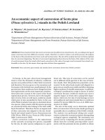
of them being what one would expect. Firstly, higher site in-
dices have shorter rotation lengths. Secondly, the higher is the
number of trees per hectare the longer are the optimal rotation
lengths. Thirdly, increasing discounting rate shortens optimal
rotation lengths (Fig. 2). The model also describes interactions
between variables. The model suggests that increasing price
of grade II (18 cm < d ≤ 35 cm) shortens optimal rotations,
which is logical [27]. However, the effect depends on the price
of grade I (d > 35 cm) so that improving P
I
partly cancels
the effect of P

II
.Theeffect of the price of grade I depends on
discounting rate: with low rates a high value of price I leads
to longer optimal rotation lengths but the opposite is true with
high rates (Fig. 3).
792 M. Pasalodos-Tato, T. Pukkala
Table II. Regression coefficients of Equation (14), (15) and (16), their standard errors (S.E.) and statistical significance.
Variable Parameter Coefficient S.E. tstatistic Significance (p)
Equation (14)
Constant a
0
4.391 0.032 138.754 < 0.0005
ln(SI)a
1
–0.394 0.003 –147.843 < 0.0005
ln(N)a
2
0.195 0.004 47.759 < 0.0005
ln(r)a
3
–0.101 0.004 –23.178 < 0.0005
P
II
a
4
–0.009 0.000 –51.636 < 0.0005
P
I
× P
II

a
5
5.38×10
−5
0.000 34.498 < 0.0005
P
I
× r a
6
–0.001 0.000 –25.697 < 0.0005
Equation (15)
Constant a
0
–7.901 0.096 –82.388 < 0.0005
SI a
1
0.083 0.001 90.242 < 0.0005
ln(T)a
2
3.110 0.018 173.338 < 0.0005
T × r a
3
–0.002 0.000 –34.645 < 0.0005
P
I
a
4
0.006 0.000 24.398 < 0.0005
P
I

× P
II
a
5
–2.98×10
−5
0.000 –8.689 < 0.0005
Fst a
6
2.337 0.013 115.100 < 0.0005
Snd a
7
1.548 0.012 66.948 < 0.0005
Trd a
8
0.776 0.000 24.398 < 0.0005
Equation (16)
Constant a
0
–20.719 1.982 –10.452 < 0.0005
SI a
1
0.132 0.016 8.054 < 0.0005
ln(T)a
2
3.717 0.485 7.657 < 0.0005
G
before
a
3

0.830 0.010 84.062 < 0.0005
T × r a
4
–0.025 0.001 –28.113 < 0.0005
P
I
a
5
0.039 0.003 12.002 < 0.0005
P
I
× P
II
a
6
–2.81×10
−4
0.000 –6.337 < 0.0005
Fst a
7
4.162 0.380 10.954 < 0.0005
Snd a
8
3.039 0.092 11.212 < 0.0005
Trd a
9
1.562 0.182 8.585 < 0.0005
SI 24
SI 18
SI 12

SI 6
0
20
40
60
80
100
120
140
0123456
Discounting rate (%)
Rotation length (years)
Figure 2. Effect of discounting rate and site index (SI) on the rotation
length when planting density is 2000 ha
−1
and prices for grades I and
II are 90 and 50 e m
−3
, respectively.
The shortest rotations are obtained when the price of grade I
and the number of trees per hectare are low (65 e m
−3
and
1000 trees per hectare, respectively) and the price of grade II
and discounting rate are high (65 e m
−3
and 5%).
3.2. Pre- and post-thinning basal area
The models obtained for stand basal area before and after a
thinning treatment in the optimal management schedules were:


G
before
= a
0
+ a
1
SI + a
2
ln(T ) + a
3
(T × r)
+ a
4
P
I
+ a
5
(P
I
× P
II
) + a
6
Fst + a
7
Snd + a
8
Trd (15)
G

after
= a
0
+ a
1
SI + a
2
ln(T ) + a
3
G
before
+ a
4
(T × r)
+ a
5
P
I
+ a
6
(P
I
× P
II
) + a
7
Fst + a
8
Snd + a
9

Trd (16)
where T is stand age expressed in years. The R
2
for Equa-
tion (15) was 0.866 and the standard error was 0.357. For
Equation (16) the R
2
was 0.897 and the standard error was
4.570. All the predictors were significant according to the t
test (p < 0.0005). Furthermore, no significant multicollinear-
ity was observed between the variables in the models.
Since the basal area of pre- and post-thinning stand was in-
fluenced by the number of the thinning, dummy variables Fst,
Snd and Trd, which represent the first, second and third thin-
ning, respectively, were included in the models. A value of 1
indicates “presence”. For example, Fst is equal to one when
Optimal management of Pinus sylvestris in Galicia 793
P
II
=65 €m
-3
5%
3%
2%
1%
0.50%
0
20
40
60

80
100
120
40 60 80 100 120 140
P
I
(€m
-3
)
Rotation length (years)
P
I
=120 €m
-3
5%
3%
2%
1%
0.50%
0
20
40
60
80
100
120
20 30 40 50 60 70 80
P
II
(€m

-3
)
Rotation length (years)
P
II
=50 €m
-3
5%
3%
2%
1%
0.50%
0
20
40
60
80
100
120
40 60 80 100 120 140
P
I
(€m
-3
)
Rotation length (years)
P
I
=65 €m
-3

5%
3%
2%
1%
0.50%
0
20
40
60
80
100
120
20 30 40 50 60 70 80
P
II
(€m
-3
)
Rotation length (years)
P
II
=35 €m
-3
5%
3%
2%
1%
0.50%
0
20

40
60
80
100
120
40 60 80 100 120 140
P
I
(€m
-3
)
Rotation length (years)
P
I
=90 €m
-3
5%
3%
2%
1%
0.50%
0
20
40
60
80
100
120
20 30 40 50 60 70 80
P

II
(€m
-3
)
Rotation length (years)
Figure 3. Effect of timber prices and discounting rate on the optimal rotation length when planting density is 2000 ha
−1
and site index is 18 m.
calculating the pre- or post-thinning basal area for the first
thinning, otherwise Fst is zero. As there were four thinnings
in the optimal management schedules, results for the fourth
thinning are obtained when all the dummy variables are zero.
Also these models include products of predictors which
were found to have interaction. This is the case for discounting
rate and age, the effect of discounting rate depending on the
age of the stand: the older the stand is, the more increasing dis-
counting rate decreases optimal pre-thinning stand basal area
(see Fig. 4). The positive coefficient of ln(T ) indicates that the
basal area before certain thinning (e.g. the second) increases
with stand age. However, age also affects through T × r, with a
consequence that the optimal pre-thinning basal area increases
less with stand age when discounting rate increases (Fig. 4).
Taking into account that the pre-thinning basal areas decrease
when the number of the thinning increases (Tab. II and Fig. 4)
the stand basal area should in most cases be decreased towards
the end of the rotation.
The model also shows that better sites indexes have higher
optimal pre-thinning basal areas, which is logical (see Fig. 5).
Planting density does not affect the optimal pre-thinning basal
area.

The price of grade III is not a significant predictor in this
model but prices of grades I and II are. The higher is the
price of grade I, the higher is the optimal pre-thinning basal
area, which means that the thinning takes place later (Fig. 6).
However, the price of grade I interacts with the price of
grade II so that increasing price II decreases the effect of price
I and the optimal pre-thinning basal area. For a given value
of price I, higher values of price II lead to earlier thinnings.
794 M. Pasalodos-Tato, T. Pukkala
BEFORE FIRST THINNING
5%
3%
2%
1%
0.50%
0
10
20
30
40
50
60
70
80
90
100
020406080100120
Stand age (years)
Basal area (m
2

ha
-1
)
AFTER FIRST THINNING
5%
3%
2%
0.50%
1%
0
10
20
30
40
50
60
70
80
90
100
020406080100120
Stand age (years)
Basal area (m
2
ha
-1
)
BEFORE SECOND THINNING
1%
0.50%

2%
3%
5%
0
10
20
30
40
50
60
70
80
90
100
020406080100120
Stand age (years)
Basal area (m
2
ha
-1
)
AFTER SECOND THINNING
0.50%
1%
2%
5%
3%
0
10
20

30
40
50
60
70
80
90
100
0 20406080100120
Stand age (years)
Basal area (m
2
ha
-1
)
BEFORE THIRD THINNING
0.50%
1%
5%
3%
2%
0
10
20
30
40
50
60
70
80

90
100
020406080100120
Stand age (years)
Basal area (m
2
ha
-1
)
AFTER THIRD THINNING
5%
2%
1%
3%
0.50%
0
10
20
30
40
50
60
70
80
90
100
0 20 40 60 80 100 120
Stand age (years)
Basal area (m
2

ha
-1
)
BEFORE FOURTH THINNING
0.50%
5%
3%
2%
1%
0
10
20
30
40
50
60
70
80
90
100
0 20406080100120
Stand age (years)
Basal area (m
2
ha
-1
)
AFTER FOURTH THINNING
2%
1%

0.50%
5%
3%
0
10
20
30
40
50
60
70
80
90
100
0 20406080100120
Stand age (years)
Basal area (m
2
ha
-1
)
Figure 4. Effect of discounting rate on the optimal stand basal area before and after thinning when site index is 18 m and timber prices for
grades I, II and III are 90, 50 and 18 e m
−3
, respectively.
Optimal management of Pinus sylvestris in Galicia 795
BEFORE; SI = 6m
4
th
thinning

2
nd
thinning
1
st
thinning
3
rd
thinning
0
10
20
30
40
50
60
70
80
90
100
020406080100120
Stand age (years)
Basal area (m
2
ha
-1
)
AFTER; SI = 6 m
4
th

thinning
3
rd
thinning
1
st
thinning
2
nd
thinning
0
10
20
30
40
50
60
70
80
90
100
020406080100120
Stand age (years)
Basal area (m
2
ha
-1
)
BEFORE; SI = 12 m
1

st
thinning
2
nd
thinning
3
rd
thinning
4
th
thinning
0
10
20
30
40
50
60
70
80
90
100
020406080100120
Stand age (years)
Basal area (m
2
ha
-1
)
AFTER; SI = 12 m

4
th
thinning
3
rd
thinning
2
nd
thinning
1
st
thinning
0
10
20
30
40
50
60
70
80
90
100
020406080100120
Stand age (years)
Basal area (m
2
ha
-1
)

BEFORE; SI = 18 m
1
st
thinning 2
nd
thinning
3
rd
thinning
4
th
thinning
0
10
20
30
40
50
60
70
80
90
100
020406080100120
Stand age (years)
Basal area (m
2
ha
-1
)

AFTER; SI = 18 m
4
th
thinning
3
rd
thinning
1
st
thinning 2
nd
thinning
0
10
20
30
40
50
60
70
80
90
100
0 20406080100120
Stand age (years)
Basal area (m
2
ha
-1
)

BEFORE; SI = 24 m
4
th
thinning
3
rd
thinning
2
nd
thinning
1
st
thinning
0
10
20
30
40
50
60
70
80
90
100
020406080100120
Stand age (years)
Basal area (m
2
ha
-1

)
AFTER; SI = 24 m
1
st
thinning
4
th
thinning
3
rd
thinning
2
nd
thinning
0
10
20
30
40
50
60
70
80
90
100
020406080100120
Stand age (years)
Basal area (m
2
ha

-1
)
Figure 5. Basal area before and after thinning for different site indices with 2% discounting rate and timber prices for grades I, II and III are
90, 50 and 18 e m
−3
, respectively.
BEFORE
4
th
thinning
3
rd
thinning
2
nd
thinning
1
st
thinning
0
10
20
30
40
50
60
70
80
90
100

020406080100120
Stand age (years)
Basal area (m
2
ha
-1
)
120 €m
-3
65 €m
-3
AFTER
1
st
thinning
2
nd
thinning
3
rd
thinning
4
th
thinning
0
10
20
30
40
50

60
70
80
90
100
0 20406080100120
Stand age (years)
Basal area (m
2
ha
-1
)
120 €m
-3
65 €m
-3
Figure 6. Effect of timber price of grade I on the stand basal area before and after thinning when discounting rate is 2%, site index is 18 m, and
timber prices of grades II and III are 50 and 18 e m
−3
, respectively.
796 M. Pasalodos-Tato, T. Pukkala
1.00
1.01
1.02
1.03
1.04
1.05
1.06
0 20406080100120
Stand age (years)

Dafter/Dbefore
Figure 7. Correlation between stand age and the ratio of the mean
diameter between post- and pre-thinning stand.
However, the effect of timber prices on the timing and inten-
sity of thinnings is rather small.
The optimal basal area after thinning is strongly dependent
on the basal area before thinning (Eq. (16), Tab. II). Other pre-
dictors are also included in the model, but their effect is much
smaller. These predictors are the same as in the model for pre-
thinning basal area. Therefore, for better site indices the basal
area after thinning is higher than for the poorer ones (Fig. 4).
Predictors T × r and ln(T)have the same effect as in the pre-
vious model. Stand basal area after a certain thinning, e.g. the
first, increases with increasing age.
The ratio of the mean diameter between post- and pre-
thinning stands (D
after
/D
before
) was also studied. The mean
value of the ratio between diameter after and before thinning
was 1.03. This ratio correlates with several parameters, for in-
stance with the stand age. At young ages thinnings tend to
be low thinnings but as stand age increases the thinnings are
more and more systematic (Fig. 7). The following equation
describes this relationship:
D
after
/D
before

= exp(0.124 − 0.025ln(T )) (17)
4. DISCUSSION
All the results of this study are based on the assumption that
the growth and yield model developed for Dieguez-Aranda
et al. [11] for even-aged Pinus sylvestris stands is correct and
works properly. Therefore, it is important to remark that the
model has some limitations in its application range due to the
nature of the data used to build the model and the properties of
the functions that composed it. The model was based on two
measurements of 91 plots that represent stands ages between
15 and 55–60 years and site indices between 7 and 24 m at
40 years. The oldest plots were only 60 years old. Therefore
our results are partly based on extrapolations of the models.
However, these extrapolations are supposed to be reasonable
because the functions used in growth and yield modelling are
robust and widely tested and follow the overall patterns of
stand development. Because well established and reasonably
simple model forms were used in growth and yield modelling,
it may be expected that no drastic deterioration in simulation
4
th
thinning
3
rd
thinning
2
nd
thinning
1
st

thinning
Optimal rotation
length given by
the model
0
10
20
30
40
50
60
70
80
0 20 40 60 80 100 120
Stand age (years)
Basal area (m
2
ha
-1
)
Figure 8. Comparison between the range of basal area before (thin
solid line) and after (dashed line) thinning obtained from the model
and the optimal management schedule (thick line) obtained in the op-
timisations for plantation density 1500 trees per hectare, discounting
rate 2%, site index 18 m, and timber prices of grades I, II and III are
90, 50 and 18 e m
−3
, respectively.
quality occurred when the limits of the modelling data were
passed.

One shortcoming of the growth models is that they have
been developed without taking into account the effect of thin-
nings on the growth of stand basal area. Therefore, the reliabil-
ity of the projections done after thinning may be questioned.
On the other hand, some studies on Scots pine suggest that the
post-thinning growth of trees can be predicted reliably without
using variables that describe the thinning [31]. In addition, the
models that we used are the only available for Scots pine in
Galicia.
Regarding the rotation length model, the first thing that at-
tracts attention is the fact that, for certain combinations of eco-
nomic and stand variables, much shorter rotations were ob-
tained than the ones traditionally used. The results obtained
show that for the very best soil qualities the optimal rotations
vary between 42 and 99 years, depending on the plantation
density, timber prices and discounting rates. For a discounting
rate of 2% the rotation length varies between 52 and 77 years
depending on plantation density and timber prices. When the
discounting rate is 5%, rotation lengths vary between 42 and
60 years depending also on the planting density and timber
prices. For the poorest site index the rotations are between 73
and 170 years, depending again on the plantation density, tim-
ber prices and discounting rates. For instance, a 2% discount-
ing rate would lead to rotation lengths between 90 and 133 and
between 73 and 104 years for a 5% discounting rate, in both
cases depending on plantation density and timber prices.
With low discounting rates a good price of timber grade I
led to long optimal rotations but with high discounting rates
the optimal rotations shortened with improving price of
grade I. This can be explained so that with high discount-

ing rates the high opportunity cost of large trees dominates,
whereas with lower rates the time matters less and improving
price of large stems makes it worthwhile to wait until more
trees reach large dimensions.
Optimal management of Pinus sylvestris in Galicia 797
FIRST THINNING
5%
3%
2%
1%
0.50%
0
5
10
15
20
25
30
35
40
45
50
020406080100120
Stand age (years)
Removed basal area (%)
SECOND THINNING
5%
3%
2%
1%

0.50%
0
5
10
15
20
25
30
35
40
45
50
020406080100120
Stand age (years)
Removed basal area (%)
THIRD THINNING
5%
3%
2%
1%
0.50%
0
5
10
15
20
25
30
35
40

45
50
020406080100120
Stand age (years)
Removed basal area (%)
FOURTH THINNING
5%
3%
2%
1%
0.50%
0
5
10
15
20
25
30
35
40
45
50
020406080100120
Stand age (years)
Removed basal area (%)
Figure 9. Dependence of thinning intensity on stand age and discounting rate when site index is 18 m and timber prices of grades I, II and III
are 90, 50 and 18 e m
−3
, respectively.
The optimal management schedules did not fit exactly

with the graphs obtained by using the models (Fig. 8). One
explanation may be that the optimisation algorithm does not
always converge to the global optimum but to a local one that
often is nearly as good as the global optimum. Rather different
management schedules may lead to very similar soil expec-
tation values. It can also happen that two quite different op-
timal management schedules are obtained with only a small
change in site index, planting density, discounting rate, or tim-
ber price. These two schedules represent different strategies
which are almost exactly good. This kind of high sensitiv-
ity of optimal management to economic parameters or stand
characteristics decreases the fitting statistics of the models for
optimal rotation and thinning basal area. Anyhow, the fitting
statistics of the models are good despite these discrepancies,
and the models guarantee, when used in forestry practise, that
the timing and intensity of cuttings are always close to the op-
timum.
The pre- and post-thinning models can be also employed
to compute the intensity of thinnings along the rotation of the
stands. The graphs obtained (Fig. 9) show that the thinning
intensity depends on the number of the thinning, the intensity
increasing from the first thinning to the fourth. The intensity of
the first thinning is around 20% of basal area, and in the fourth
around 30% of basal area. Furthermore, thinning intensity in-
creases with the increment of discounting rate and decreases
with the increasing age.
The results obtained in this study are quite similar to the
ones that Palahí and Pukkala [25] obtained for even-aged Pi-
nus sylvestris stands in Catalonia (north-eastern Spain). They
optimised the management schedule using the same method,

namely Hooke and Jeeves algorithm, and the same objective
variable (LEV) as in the study. They found out that five thin-
nings were needed to maximise the LEV. The rotation lengths
were longer than the ones achieved in the present study. These
differences are due to the fact that the growth rates for Pinus
sylvestris in Catalonia are much lower than in Galicia.
The models can be used in forestry practise as follows: the
age of a stand is compared to the model for optimal rotation
length (Eq. (14)). If the stand is older than the optimal rotation
age, the stand is to be clear-felled. Otherwise the stand basal
area is compared to the pre-thinning basal area given by Equa-
tion (15). If the stand basal area exceeds the model prediction,
the stand should be thinned. The optimal post-thinning basal
area is obtained from Equation (16). Various diagrams (e.g.
Figs. 2 and 5) or software products can be prepared from the
models to further ease their use in forestry practice.
Acknowledgements: The research reported in this paper was sup-
ported by Fundación Barrié de la Maza (Spain).
798 M. Pasalodos-Tato, T. Pukkala
REFERENCES
[1] Ambrosio Y., Tolosana E., Vignote S., El coste de los trabajos de
aprovechamiento forestales como factor condicionante de la gestión
forestal. Aplicación a las cortas de mejora en masas de pino sil-
vestre, in: Rojo A. et al. (Eds.), Actas del Congreso de Ordenación
y Gestión Sostenible de Montes. Santiago de Compostela, 4–9 de
octubre 1999, edición CD.
[2] Arenas S.G., Rojo A., Cortas de mejora en repoblaciones de Pinus
sylvestris L. de la Comarca Montaña de Lugo, in: Vignote S.
(Ed.), Cortas de Mejora de las Masas Españolas: Selvicultura,
Aprovechamientos y Comercialización de los Productos, Fundación

Conde del Valle de Salazar, 1998, pp. 61–70.
[3] Bazaraa M.S., Shetty C.M., Nonlinear programming: theory and al-
gorithms, John Wiley & Sons, New York, 1979.
[4] Bravo F., Díaz-Balteiro L., Evaluation of new silvicultural alter-
natives for Scots pine stands in northern Spain, Ann. For. Sci. 61
(2004) 163–169.
[5] Clutter J.L., Fortson J.C., Pienaar L.V., Brister G.H., Bailey R.L.,
Timber management: a quantitative approach, John Wiley & Sons,
New York, 1983.
[6] DGCONA, Tercer Inventario Forestal Nacional (1.997-2.006):
Galicia, Dirección General de Conservación de la Naturaleza,
Ministerio de Medio Ambiente, Madrid, 2002.
[7] Díaz-Balteiro L., Romero C., Modelling timber harvest scheduling
problems with multiple criteria: an application in Spain, For. Sci. 44
(1998) 47–57.
[8] Díaz-Balteiro L., Romero C., Forest management optimisation
models when carbon captured is considered: a goal programming
approach, For. Ecol. Manage. 174 (2003) 447–457.
[9] Díaz-Balteiro L., Álvarez Nieto A., Oria de Rueda Salgueiro
J.A., Integración de la producción fúngica en la gestión forestal.
Aplicación al monte “Urcido” (Zamora), Invest. Agrar.: Sist. Recur.
For. 12 (2003) 5–19.
[10] Dieguez-Aranda U., Castedo Dorado F., Álvarez González J.G.,
Funciones de crecimiento en área basimétrica para masas de Pinus
sylvestris L. procedentes de repoblación en Galicia, Invest. Agrar.:
Sist. Recur. For. 14 (2005) 253–266.
[11] Dieguez-Aranda U., Castedo Dorado F., Álvarez González J.G.,
Rojo Alboreca A., Dynamic growth model for Scots pine (Pinus
sylvestris L.) plantations in Galicia (north-western Spain), Ecol.
Model. 191 (2006) 225–242.

[12] Fang Z., Borders B.E., Bailey R.L., Compatible volume-taper mod-
els for loblolly and slash pine based on a system with segmented-
stem form factors, For. Sci. 46 (2000) 1–12.
[13] Gonzalez J.R., Pukkala T., Palahí M., Optimising the management
of Pinus sylvestris L. stand under the risk of fire in Catalonia (north-
east Spain), Ann. For. Sci. 62 (2005) 493–501.
[14] Hasenauer H., Burkhart H.E., Amateis R.L., Basal area develop-
ment in thinned and unthinned loblolly pine plantations, Can. J. For.
Res. 27 (1997) 265–271.
[15] Hooke R., Jeeves T.A., “Direct Search” solution of numerical and
statistical problems, J. Assoc. Comput. Mach. 8 (1961) 212–229.
[16] Hyytiäinen K., Integrating economics and ecology in stand-level
timber production, Finnish Forest Research Institute, Research
Papers 908, 2003, 42 p.
[17] Kuliesis A., Saladis J., The effect of early thinning on the growth of
pine and spruce stands, Baltic. For. 4 (1998) 8–16.
[18] Mäkinen H., Isomäki A., Thinning intensity and growth of Scots
pine stands in Finland, For. Ecol. Manage. 201 (2004) 311–325.
[19] Mäkinen H., Isomäki A., Thinning intensity and long-term changes
in increment and stem form of Scots pine trees, For. Ecol. Manage.
203 (2004) 21–34.
[20] Mäkinen H., Isomäki A., Hongisto T., Effect of half-systematic and
systematic thinning on the increment of Scots pine and Norway
spruce in Finland, Forestry 79 (2006) 103–121.
[21] Martínez E., Rodríguez-Soalleiro R., Rojo A., Análisis de la
selvicultura desarrollada en los montes de Pinus sylvestris L. de
Galicia. Perspectivas futuras, in: II Congreso Forestal Español, Irati,
Gobierno de Navarra, Tomo IV, 1997, pp. 387–392.
[22] Miina J., Preparation of management models using simulation and
optimisation, in: Pukkala T., Eerikäinen K. (Eds.), Tree seedling

production and management of plantation forests, University of
Joensuu, Faculty of Forestry, Research Notes 68, 1998, pp. 165–
180.
[23] Møller C.M., The influence of thinning on volume growth. Part I,
in: Heiberg S.O. (Ed.), Thinning problems and practise in Denmark,
Technical Publication No. 76, State University of New York,
College of Forestry, 1954, pp. 5–32.
[24] Montero G., Cañellas I., Ortega C., Del Río M., Results from a thin-
ning experiment in a Scots pine (Pinus sylvestris L.) natural regen-
eration stand in the Sistema Ibérico mountain range (Spain), For.
Ecol. Manage. 145 (2001) 151–161.
[25] Palahí M., Pukkala T., Optimising the management of Scots pine
(Pinus sylvestris L.) stands in Spain based on individual-tree mod-
els, Ann. For. Sci. 60 (2003) 105–114.
[26] Petterson N., The effect of density after precommercial thinnings
on volume and structure in Pinus sylvestris and Picea abies stands,
Scand. J. For. Res. 8 (1993) 528–539.
[27] Pukkala T., Puun hinta ja taloudellisesti optimaalinen hakkuun
ajankohta, Metsätieteen aikakauskirja 1 (2006) 33–48.
[28] Pukkala T., Mabvurira D., Optimising the management of
Eucalyptus grandis plantations in Zimbabwe. in: Pukkala T.,
Eerikäinen K. (Eds.), Growth and yield modelling of tree planta-
tions in South and East Africa, University of Joensuu, Faculty of
Forestry, Research Notes 97, 1999, pp. 113–123.
[29] Pukkala T., Miina J., Kellomäki S., Response to different thinning
intensities in young Pinus sylvestris, Scand. J. For. Res. 13 (1998)
141–150.
[30] Pukkala T., Miina J., Rautianen O., Dependence of stand manage-
ment on management goal, in: Pukkala T., Eerikäinen K. (Eds.),
Tree seedling production and management of plantation forest,

University of Joensuu, Faculty of Forestry, Research Notes 68,
1998, pp. 165–180.
[31] Pukkala T., Miina J., Palahí M., Thinning response and thinning
bias in a young Scots pine stand, Silva Fenn. 36 (2002) 827–840.
[32] Rodriguez-Soalleiro R., Vega P., Apuntes de selvicultura de zonas
atlánticas, Unicopia, Lugo, Spain, 1998.
[33] Rojo A., Diéguez-Aranda U., Rodríguez Soalleiro R., Gadow K.v.,
Modelling silvicultural and economic alternatives for Scots pine
(Pinus sylvestris L.) plantations in north-western Spain, Forestry 78
(2005) 385–401.
[34] Salminen H., Varmola M., Development of Scots pine stands
from precommercial thinning to first commercial thinning, Folia
Forestalia 752 (1990) (in Finnish with English summary).
[35] Trasobares A., Pukkala T., Optimising the management of uneven-
aged Pinus sylvestris L. and Pinus nigra Arn. mixed stands in
Catalonia, north-east Spain, Ann. For. Sci. 61 (2004) 747–758.
[36] Valsta L.T., Stand management optimization based on growth simu-
lators, The Finnish Forest Research Institute, Research Papers 453,
1993, pp. 51–81.
[37] Varmola M., Salminen H., Timing and intensity of precommercial
thinning in Pinus sylvestris stands, Scand. J. For. Res. 19 (2004)
142–151.
[38] Xunta de Galicia, O monte galego en cifras, Dirección Xeral de
Montes e Medio Ambiente Natural, Santiago de Compostela, 2001.
[39] Xunta de Galicia, Anuario de Estatística Agraria 2003, Consellería
de Medio Rural, 2006.