Báo cáo lâm nghiệp: " A state-space approach to stand growth modelling of European beech" pot
Bạn đang xem bản rút gọn của tài liệu. Xem và tải ngay bản đầy đủ của tài liệu tại đây (480.93 KB, 10 trang )
Ann. For. Sci. 64 (2007) 365–374 Available online at:
c
INRA, EDP Sciences, 2007 www.afs-journal.org
DOI: 10.1051/forest:2007013
Original article
A state-space approach to stand growth modelling of European beech
Thomas N-L
*
,VivianK.J
Forest & Landscape, Denmark, Copenhagen University, Hørsholm Kongevej 11, DK-2970 Hørsholm, Denmark
(Received 7 September 2006; accepted 20 December 2006)
Abstract – Static models of forest growth, such as yield tables or cumulative growth functions, generally fail to recognize that forest stands are dynamic
systems, subject to changes in growth dynamics due to silvicultural interventions or natural dynamics. Based on experimental data, covering a wide
range of initial spacings and thinning practises, we developed a dynamic stand growth model of European beech in Denmark. The model entailed
three equations for predicting dominant height growth, basal area growth, and mortality. The signs of the parameter estimates generally corroborated
the anticipated growth paths of dominant height and basal area. Although statistical tests indicated significant systematic deviations between observed
and predicted values, the deviations were small and of little practical importance. Cross validation procedures indicated that the model may be applied
across a wide range of growth conditions and thinning practises without significant loss of precision.
difference equation / dominant height / basal area / stem number / Fagus sylvatica L.
Résumé – Une approche état-espace de la modélisation de la croissance des peuplements de hêtre. Les modèles statiques de croissance des
peuplements forestiers, tels que les tables de production ou les fonctions cumulatives de croissance, ne reconnaissent pas que les peuplements forestiers
sont des systèmes dynamiques, soumis à des changements de dynamiques de croissance dus aux interventions sylvicoles ou à des dynamiques naturelles.
Sur la base de données expérimentales, couvrant un large éventail d’espacements initiaux et de pratiques d’éclaircie, nous avons développé un modèle
dynamique de croissance de peuplement pour le hêtre au Danemark. Le modèle comporte trois équations pour prédire la croissance de la hauteur
dominante, la croissance de la surface terrière et la mortalité. Les signes des paramètres estimés ont confirmé en général la trajectoire prévue de la
croissance de la hauteur dominante et de la surface terrière. Bien que les tests statistiques aient indiqué des déviations systématiques significatives entre
valeurs observées et valeurs prédites, les déviations ont été faibles et de peu d’importance pratique. Des procédures de validation croisées ont indiqué
que le modèle peut être appliqué dans un large éventail de conditions de croissance et de pratiques sylvicoles sans perte significative de précision.
équation aux différences / hauteur dominante / surface terrière / nombre de troncs / Fagus sylvatica L.
1. INTRODUCTION
Fitting of simple growth curves for prediction of stand level
variables such as average height, stand basal area or stem num-
ber is an old discipline in forest growth modelling [3,7,17,30].
Such models describe the course of stand variables over time
and may yield reasonable estimates in many situations. How-
ever, these static models generally fail to recognize that forest
stands are dynamic systems, subject to sudden changes caused
by silvicultural interventions or natural dynamics. As the in-
tensity of management increases, interventions may vary in
timing and intensity and the stand variables may follow a po-
tentially infinite number of paths [15].
Dynamic systems subject to environmental change may be
modelled using the state-space approach. The state-space ap-
proach relies on the assumption that the state of a system at
any given time contains the information needed to predict the
behaviour of the system in the future [15]. Hence, the state
of a system may be viewed as the cumulated information of
the past, and only information on the present is needed to pre-
dict the future behaviour of the system. Change (increment
or mortality) is modelled from the state of the system at any
* Corresponding author:
point in time and any future state is predicted from the cur-
rent state and current and future actions through iteration. The
state-space approach in this sense is closely related to the con-
cept of control theory, and is adequate for modelling systems
subject to control (i.e. environmental changes) with feed back
because explicit modelling of the complex relation between
interventions and responses of the system is avoided.
Covering 17% of the total forest area European beech is the
most common deciduous species in Denmark [26] and also
one of the most significant in economic terms. Current mod-
els for predicting stand level growth of beech in Denmark are
standard yield tables based on graphical smoothing of perma-
nent sample plot data [21,34]. Despite the practical importance
of these tables, the methods applied in their construction have
generally lacked statistical rigour and objectivity. The aim of
this study was to develop a stand level model for predicting the
growth of even-aged stands of European beech. The main fo-
cus was the development of dynamic models based on a state-
space approach.
2. MATERIALS AND METHODS
The data potential for developing stand level models for beech
comprised 60 permanent, even-aged and mono-specific spacing,
Article published by EDP Sciences and available at or />366 T. Nord-Larsen, V.K. Johannsen
species and thinning experiments in beech including a total of 149
individual plots. Plot sizes varied between 0.07 and 2.65 ha with an
average of 0.40 ha. The experiments were located in most parts of
Denmark and covered a wide range of different site types and growth
conditions. The data was collected during the years 1872 to 2005 and
the stands were observed for 10 to 120 years. The number of mea-
surement occasions totalled 2065.
The data included a wide range of different treatments in terms of
initial spacing and thinning practices from unthinned control plots to
heavily thinned plots. In the thinning experiments, the treatments in-
cluded A-, B-, C-, and D-grade thinnings, and in some cases even
heavier thinnings. Usually, the D-grade is thinned to a basal area
of 50% relative to the unthinned control (A-grade). The B- and
C-grades are intermediate, dividing the interval between A-and D-
grades equally. Some plots were managed according to other thin-
ning strategies, such as group- or selection-thinning and others were
managed according to the thinning strategy typical at the time.
In the majority of plots, all trees were numbered, marked perma-
nently at breast height (1.3 m) and recorded individually. In 451 mea-
surements carried out before 1930 and in some very young stands
with high stem numbers, trees were recorded in tally lists to 1-cm
diameter classes (before 1901 to 1-inch classes). Also in 13 very
young stands with high stem numbers, only a subset of stems were
measured, e.g. every fifth or tenth row. Breast height diameters were
obtained by averaging two perpendicular calliper readings. Observa-
tions also included records on whether the tree was alive or dead at the
time of measurement. Total height was typically measured for about
30 trees per plot on each measurement occasion. Finally, soil texture
analyzes were carried out in 48 experiments, providing information
on percentages of clay, silt, fine sand and coarse sand in the top one
metre of the mineral soil.
2.1. Basic calculations
Based on paired observations of diameter and height, height-
diameter equations were estimated for each plot and measurement
occasion using a modified Näslund-equation [24, 36]:
h
ij
= 1.3 +
d
ij
α + β · d
ij
3
+ ε
ij
(1)
where d
ij
is diameter at breast height and h
ij
is total tree height of the
ith tree and jth plot and measurement occasion. α and β are parame-
ters to be estimated and ε is the error term. The equations were used
to estimate the height of trees not measured. Dominant height, H
100
(m), defined as arithmetic mean height of the 100 thickest trees per
hectare was subsequently calculated for each plot and measurement
combination. In the few cases where stem numbers were less than
100 per hectare, H
100
was estimated as the arithmetic mean height.
Differences in plot size affect dominant height estimates, leading to
underestimation on small plots. However, as there is no correlation
between treatment and plot size (plots with many stems per hectare
are not generally smaller than plots with few stems per hectare), there
are no systematic effects of the choice of plot sizes. Further, although
the span of plot sizes seem large, the majority of plots are approxi-
mately the same size (0.25–0.5 ha).
Stem numbers, N (100 ha
−1
) were calculated as the number of
individual trees per hectare taller than 1.3 m. When trees forked be-
low 1.3 m, each stem was measured individually but multiple stems
from the same root were counted as one tree. Within the research
Table I. Summary statistics of dominant height (H
100
), basal area (G),
stem number (N), quadratic mean diameter (D
g
)andage(T ).
Variable Unit N Mean Minimum Maximum Std. Dev.
H
100
m 1458 20.88 5.08 36.95 7.69
G m
2
ha
−1
1458 20.04 0.21 73.58 8.92
N ha
−1
1458 1372 0.49 24720 2317
D
g
cm 1458 26.72 2.70 82.85 17.56
T years 1458 60.70 14 200 47.65
plots, trees were typically separated into over- and understorey and
the understorey was measured less intensively than the overstorey.
Understorey trees were excluded from this analysis.
Stand basal area, G (m
2
ha
−1
), of each plot was estimated by
summation of individual tree basal areas calculated from the diam-
eter measurements. When trees were recorded in tally lists, the mid-
diameter of each class was used as an estimate of the diameter of
all trees in that class. Quadratic mean diameter, D
g
(cm), was de-
rived from the estimates of N and G. The data represent a wide range
of stand ages and stand values such as H
100
, G, N, and D
g
(Tab. I,
Fig. 1).
2.2. Model development
Any number of stand variables may be chosen to describe stand-
level growth. The choice depends on the desired level of resolution
and the practical application. Among the most commonly used vari-
ables in stand level models are H
100
, G, N, D
g
, and stand volume (V)
and their derivatives. Since D
g
and V may be derived from the first
three variables, the models in this study included H
100
, G,andN.
The model form used to describe the development of different
variables essentially depends on the modelling subject and a great
variety of model forms have been presented for various forestry ap-
plications. Forest growth dynamics are often characterized by an ini-
tial expansion followed by a dampening effect and may adequately
be described with a sigmoid model form. Among the most well
known sigmoid models are the mono-molecular [33], logistic [45,46],
Gompertz [16], Bertalanffy [2] and Richards [39] equations. Despite
the apparent diversity of growth models, [48] found that most of the
mentioned equations can be transformed into a single equation in
which the two opposing factors, initial multiplicative expansion fol-
lowed by exponential dampening are expressed as:
dy
dt
= αy
β
e
γy
(2)
where y represents the size of the modelling subject and α, β,and
γ are parameters. This equation is very similar to that of Berta-
lanffy [2], and was initially developed for predicting individual tree
growth and has in a number of studies been expanded to include a
number of additional elements such as basal area and basal area in
larger trees [18, 19, 23]. Different forms of Equation (2) have also
been used in stand growth modelling [23]. Greatly inspired by the
latter work and based on the proposition that density measured as
stand basal area affects both basal area growth and dominant height
growth, we used the following equations to describe height and basal
area growth:
dH
100,ij
dt
= α
0
H
α
1
100,ij
e
α
2
H
100,ij
+α
3
G
ij
+ ε
H,ij
(3)
Stand growth modelling of European beech 367
Figure 1. Stand-level values of H
100
, G, N,andD
g
.
dG
ij
dt
= β
0
G
β
1
ij
e
β
2
G
ij
+β
3
H
β
4
100,ij
+ ε
G,ij
, (4)
where α
0
− α
3
and β
0
− β
4
are parameters to be estimated and ε
H,ij
∼
N
0,σ
2
H
and ε
G,ij
∼ N
0,σ
2
G
are the error terms of the ith measure-
ment occasion on the jth plot.
The reduction in stem number in even-aged stands is caused by
thinning operations and mortality. When using the state-space ap-
proach, thinnings are simulated explicitly and need not be mod-
elled. Mortality may be perceived to consist of two factors: (i) simple
chance of death and (ii) a density-dependent mortality that increases
with density. We modelled the simple chance of death as a fraction
of the stem number and the density dependent reduction in stem-
numbers by the exponential of the inverse relative spacing (RS =
√
10000/N/H):
dN
ij
dt
= −γ
1
N
γ
2
ij
e
γ
3
√
N
ij
H
100,ij
+ ε
N,ij
(5)
where ε is the error term and γ
1
− γ
3
are parameters to be estimated.
Preliminary estimation of the model revealed that a simpler model
and similar fit statistics were obtained for γ
2
= 1, while ensuring a
reasonable model behaviour. Thus in the final estimation of the sys-
tem of equations, γ
2
was fixed at 1.
In Equations (3), (4) and (5) the state-space problem is formu-
lated as a continuous-time model. However, since the equations above
have no analytical solution they must be estimated numerically which
is rather cumbersome. To reduce the computational load we used a
discrete-time model in which ∆y/∆t is substituted for dy/dt:
∆H
100,ij
∆t
= α
0
H
α
1
100,ij
e
α
2
H
100,ij
+α
3
G
ij
+ ε
H,ij
(6.1)
∆G
ij
∆t
= β
0
G
β
1
ij
e
β
2
G
ij
+β
3
H
β
4
100,ij
+ FV [G]
i+1, j
+ ε
G,ij
(6.2)
∆N
ij
∆t
= −γ
1
N
γ
2
ij
e
γ
3
√
N
ij
H
100,ij
+ FV [N]
i+1, j
+ ε
N,ij
(6.3)
In the discrete model, shifts in G and N caused by thinnings or en-
vironmental hazards are formulated explicitly by “Forcing Values”,
FV[G] and FV[N] respectively.
2.3. Site-specific effects
Modelling growth and yield requires some measure of site quality
to make reasonable forecasts. In a number of studies the site-specific
effects have been included by allowing some parameters to be local
or plot-specific and others to be general or global [1, 6, 14]. Subse-
quently the local parameters may be related to site index or environ-
mental properties such as climate, elevation or soil properties, or the
parameter estimate may be perceived as an indicator of site quality
itself [23, 27, 31].
Which parameter to make local and which to make global depends
on the modelling subject. The simplest formulation of Equations (6.1)
and (6.2) emerges from leaving α
0
and β
0
to be local and the remain-
ing parameters to be global since the site-specific parameter is then a
simple factor. Preliminary studies showed similar fit statistics and ex-
trapolation properties of making α
0
and α
1
local whereas making α
2
local resulted in poorer model performance. Although the fit statistics
showed no differences between the two first formulations, making α
0
and β
0
local resulted in greater ease of fit and a simpler model as the
site specific effect is then merely a factor.
When fitting a similar system of equations, Johannsen [23] hy-
pothesized that it is possible to find an allometric relation between
the site-specific parameters of the height and basal area equations.
Hence the site-specific effect of both equations may be captured in
one rate constant (a). Preliminary studies showed that α
0
and β
0
were
highly correlated and their relation was adequately modelled by a lin-
ear model. Hence, the following system of equations was obtained:
∆H
100,ij
∆t
= a
j
H
α
1
100,ij
e
α
2
H
100,ij
+α
3
G
ij
+ ε
H,ij
(7.1)
∆G
ij
∆t
=
β
01
+ β
02
· a
j
G
β
1
ij
e
β
2
G
ij
+β
3
H
β
4
100,ij
+ FV [G]
i+1, j
+ ε
G,ij
(7.2)
∆N
ij
∆t
= −γ
1
N
γ
2
ij
e
γ
3
√
N
ij
H
100,ij
+ FV [N]
i+1, j
+ ε
N,ij
(7.3)
where α
0
in Equation (6.1) is substituted by the local parameter a and
β
0
in Equation (6.2) is substituted by a linear function of a and the
two global parameters β
01
and β
02
. The remaining parameters were
368 T. Nord-Larsen, V.K. Johannsen
estimated globally. Note that a represents a site-specific effect that
may be considered a random effect in a mixed, hierarchical model
(for an example see [20]). However, this requires that the random
effect is normally or otherwise distributed. Rather than making such
assumptions we estimated a specifically for each experiment using an
index variable method.
For practical application of the stand model, a must be estimated
from a series of observations of height and basal area. When the
model is applied where beech has not been grown before or when
there are no sequential observations of stand variables the estimation
cannot be carried out. In a preliminary study we therefore related a
to the proportion of different soil fractions (clay, silt, fine sand, and
coarse sand) in the uppermost 1 m of the soil to see if a could be
estimated from soil properties alone, but found no statistically signif-
icant correlations. However, a was highly correlated with the more
traditional measure of site quality, site index, defined as the dominant
height at age 50. To allow flexible use of the model, depending on
the available data, we also estimated the stand level model where site
specific effects were substituted by a linear function of site index (S):
∆H
100,ij
∆t
=
α
01
+ α
02
· S
j
H
α
1
100,ij
e
α
2
H
100,ij
+α
3
G
ij
+ ε
H,ij
(8.1)
∆G
ij
∆t
=
β
01
+ β
02
· S
j
G
β
1
ij
e
β
2
G
ij
+β
3
H
β
4
100,ij
+ FV [G]
i+1, j
+ ε
G,ij
(8.2)
∆N
ij
∆t
= −γ
1
N
γ
2
ij
e
γ
3
√
N
ij
H
100,ij
+ FV [N]
i+1, j
+ ε
N,ij
(8.3)
Site index was estimated for each experiment prior to fitting of the
dynamic stand model using a site equation developed for beech in
Denmark [37].
2.4. Model estimation
Different forms of the state-space approach have been used by
various authors to model individual tree or stand-level growth.
García [14] modelled height growth of even-aged stands by a stochas-
tic differential equation. The parameters were estimated simultane-
ously by a maximum-likelihood procedure that included an explicit
expression of the error term.
Instead of using continuous-time models, a number of authors
have fitted discrete-time models of individual tree and stand level
growth. Lynch and Moser [28] as well as Hein and Dhôte [20] related
average rates of change to the current state of the system (“averag-
ing method” or “difference quotient method”). Clutter [7] recognized
that the average growth rate is more likely to be closest to the actual
growth rate at the midpoint of the measurement interval and related
average changes to the interpolated state variables at the midpoint of
the observed growth interval (“midpoint method”).
Rather than assuming the growth rate to be constant and equal
to average growth throughout the growth period McDill and Am-
ateis [32] suggested that discrete time models should be fitted from
observations with any time interval using the hypothesized functional
form of the difference equation as basis for interpolation. This ap-
proach was later generalized for predicting annual growth rates for a
number of individual tree and stand level variables [4, 5, 23].
Following the approach of McDill and Amateis [32] the estimation
problem may be written as a series of annual difference equations that
increment stand height, stand basal area or stem numbers from some
initial state to the state at some later point in time, using the years
between the two observations as the number of iterations. Consider-
ing height, the state at the end of the growth period may be predicted
from the state at the beginning of the growth period by a series of
predicted annual increments:
ˆ
H
i+1, j
= H
ij
+ f
H
ij
, G
ij
(9.1)
ˆ
H
i+2, j
=
ˆ
H
i+1, j
+ f
ˆ
H
i+1, j
,
ˆ
G
i+1, j
(9.2)
.
.
.
ˆ
H
i+t, j
=
ˆ
H
i+t−1, j
+ f
ˆ
H
i+t−1, j
,
ˆ
G
i+t−1, j
, (9.3)
where f
H
ij
, G
ij
is expressed in Equation (7.1) and models annual
height increment at the jth plot at the time i + t (t = 0, 1, 2, ,n). The
parameters of the annual difference equation may then be estimated
using a nonlinear least squares procedure that minimizes the squared
deviations of
ˆ
H
i+t, j
from H
i+t, j
.
As indicated in Equation (9.1), the procedure requires some ini-
tial observation to initiate the iterations. The initial state may be ei-
ther [23]:
1. Fixed initial values;
2. The first measurement at each plot;
3. The previous measurement of each state-variable ;
4. Estimated initial values, (i) common to all observations, (ii) com-
mon to each plot or (iii) unique for each observation.
Using fixed initial values for the estimation procedure as in (1) and
(4) requires that all thinnings throughout the stands life have been
recorded to account for shifts in G and N (see Eqs. (6.2) and (6.3)).
Since unrecorded thinnings oftentimes occurred before the establish-
ment of the experiments, this option was precluded. Options (2) and
(3) both use measured values as initial conditions and avoid the prob-
lem of silvicultural activities before the initiation of the experiments.
Using the previous measurement as initial state prevents error accu-
mulation due to errors in the shift vectors and this method to a greater
extent reflects the practical application. Consequently, the estimation
procedure was carried out using option (3).
The system of equations presented in (7.1)–(7.3) is referred to as a
seemingly unrelated regression (SUR) system since only one depen-
dent variable occurs in each equation. If no error correlation exists
between the individual regressions they may be treated as indepen-
dent problems. However, if error correlations are present OLS esti-
mates are inefficient. In this study cross-equation error correlations
were included in a generalized least squares procedure using iterated
seemingly unrelated estimation (ITSUR) [41].
The data used for this study represents a structure of repeated mea-
surements on individual plots. Failure to recognize that within-plot
measurements are correlated may result in inefficient estimates and
underestimated standard errors when correlations are strong. When
growth is viewed as an incremental process where only current con-
ditions influence current growth, the problems of serial correlation
are usually avoided [14, 42]. However, we explicitly modelled the
serial correlation by including a generalized formulation of the first-
order autoregressive model that accommodates the irregular spacing
of measurements:
ε
i
= ρ
t
i
−t
i−1
m
ε
i−1
+ u
i
(i = 1, 2, , n) (10)
where ε
i
is the error at the i th measurement, t is the time, ρ
m
is the
coefficient of correlation of the mth equation and the u
i
’s are normally
and independently distributed random errors.
Stand growth modelling of European beech 369
2.5. Statistical fit of the model
Characterization and assessment of errors cannot be performed di-
rectly on the model subject since the model predicts annual incre-
ment, which is not observed directly. Instead model evaluation may
be carried out on the predicted state of the model subject at the end
of the period. However, this leads to highly inflated estimates of fit
statistics since much of the variation is explained by the initial state
of the model subject. Instead the errors may be characterized by the
deviations between predicted and observed periodic annual increment
(PAI ). The two measures were both applied in the analyzes.
Model error were first characterised in terms of magnitude and dis-
tribution by plotting residuals against predicted values of the model
subject. Furthermore, residuals were plotted against observed values
of other stand variables to expose any obvious trends. Temporal and
regional trends were evaluated by plots of residuals against measure-
ment years and natural-geographical regions of Denmark according
to Jakobsen [22].
In addition to the visual appraisal of the errors a number of sum-
mary statistics were calculated for the entire data set as well as for
different strata and initial values of the model subject. The summary
statistics include average bias (AB), average absolute bias (AAB),
root mean squared error (RMSE), R
2
-statistics and critical error con-
fidence bounds (CEB) [12, 38]. The latter provides an estimate of the
magnitude of the error that can be expected when using the model.
Statistical tests of model bias, model stability, and for the model
assumptions on patterns and distribution of the residuals, were carried
out. The statistical tests of model bias included simultaneous F-tests
for unit slope and zero intercept of the linear regression of observed
versus predicted data [9]. Predictive performance and stability of the
parameter estimates were evaluated by leave-one-out cross validation
in which entire experiments were left out of the estimation data one at
a time and subsequently the estimated model was applied to the left-
out experiment. This procedure was extended to evaluate the stability
of parameter estimates across site index, thinning practises, regions
and time of birth by iteratively leaving out different strata of data.
3. RESULTS
Parameter estimates of equations (7.1)–(7.3) and (8.1)–
(8.3) were all significant (P < 0.05) except for α
01
and β
01
,
which were both eliminated from the models. After reduction
of the models all parameters were significant. The correlation
coefficient of the height model (ρ
H
) was non-significant, indi-
cating no correlation of height growth in subsequent growth
periods. The correlation coefficient of basal area growth (ρ
G
)
was highly significant, which may indicate that basal area
growth in subsequent periods was positively correlated or may
originate from model misspecification.
The reduced model system, using the site specific param-
eter a (Eqs. (7.1)–(7.3)) accounted for more than 98% of
the observed variation of H
100
, G,andN at the end of the
growth period (Tab. II). Based on PAI the height and basal
area models explained 33% and 72% of the total variation
in annual growth, respectively, whereas the mortality model
explained 44% of the observed annual changes in stem num-
bers. Also based on PAI, average bias (AB) was very close
to 0 for all models. Average absolute bias (AAB) was 0.14 m
for the height growth model, 0.18 m
2
ha
−1
for the basal area
growth model, and 24 ha
−1
for the mortality model. Root mean
squared error (RMSE) was 0.22 m for the height growth model
(based on PAI), 0.27 m
2
ha
−1
for the basal area growth model
and 80 ha
−1
for the mortality model. Critical error confidence
bounds (CEB) was 0.42–0.44 m for the height growth model,
0.51–0.55 m
2
ha
−1
for the basal area growth model and 153–
164 ha
−1
for the mortality model. Precision and bias of sys-
tem of equations using site index (Eqs. (8.1)–(8.3)) was almost
identical to that of Equations (7.1)–(7.3).
Plots of residual PAI of H
100
, G, N and D
g
against their
corresponding predicted values revealed no obvious trends
(Fig. 2). Neither did plots of residual PAI for the three mod-
els against other stand variables (not shown). Simultaneous F-
tests did not reveal any model bias of the height and mortality
models but showed a significant bias of the basal area model.
However, the systematic deviations were small and of little
practical importance.
Residuals were approximately homogeneous with zero
mean for H
100
and G, but residual variance for N increased
with increasing stem numbers. As variance heterogeneity only
affects parameter estimates when it expresses some model
misspecification, the latter may only be important in relation
to model inference. Distributions of the residuals of the three
models all deviated significantly from normality, although a
graphical analysis indicated that deviations were small. Resid-
uals of individual experiments after correction for first-order
serial correlation had no significant correlations.
The cross-validation procedure of leaving out entire exper-
iments in the estimation resulted in only a small increase in
RMSE of the H
100
and G models (0.6% and 5.4% respectively)
but a rather large increase for the N model (61%). Further
cross-validation procedures in which different classes of data
were left out based on different characteristics (i.e. site index,
growth region, year of birth and thinning intensity) resulted in
only a small increase in RMSE, indicating a remarkable sta-
bility of the parameter estimates.
4. DISCUSSION
4.1. Parameter estimates
The signs of the parameter estimates generally corroborated
the anticipated growth paths of both H
100
and G (Tab. II). The
positive α
2
and β
2
indicates an initial multiplicative expansion
of growth followed by an exponential dampening as a result of
the negative estimates of α
3
and β
3
, the resulting growth curve
being sigmoid.
The estimate of α
4
indicates a positive response of dom-
inant height growth to increasing levels of stand density
(Fig. 3). This finding contradicts the generally accepted notion
that height growth is essentially unaffected by stand density. A
similar pattern is also observed for a number of other species
including Scots pine [13], oak [23], ash [25], jack pine and as-
pen [11]. Conversely, MacFarlane et al. [29] and DeBell and
Harrington [8] found the opposite effect of density on height
growth in loblolly pine and red alder, respectively. The spe-
cific effect is probably dependent on species, site, and stand
370 T. Nord-Larsen, V.K. Johannsen
Table II. Parameter estimates of the system of equations presented in equations (7.1)–(7.3) and (8.1)–(8.3) along with their standard errors. R
was calculated from the deviations between predicted and observed values at the end of the growth periods.
Site parameter a Site index
Model Parameter Estimate Std. err. R
2
Estimate Std. err. R
2
H
100
a 0.0281
a
0.0100
a
0.9909 – – 0.9909
α
02
–– 1.842 × 10
−3
6.06 × 10
−4
α
1
2.1092 0.1913 1.8290 0.1844
α
2
–0.1907 0.0117 –0.1791 0.0113
α
3
0.0138 0.0023 0.0145 2.18 × 10
−3
ρ
H
0.0128 0.2357 0.0143 0.2386
G β
02
31.3437 11.1644 0.9904 0.0406 5.66 × 10
−3
0.9882
β
1
0.5087 0.0744 0.5736 0.0690
β
2
–0.0125 0.0033 –0.0151 3.18 × 10
−3
β
3
–0.0175 0.0071 –0.0756 0.0240
β
4
1.3125 0.1089 0.9466 0.0797
ρ
G
0.7173 0.0178 0.7299 0.0177
N γ
1
0.0008 0.0001 0.9883 6.93 × 10
−4
1.30 × 10
−4
0.9885
γ
2
1– 1 –
γ
3
0.0342 0.0016 0.0349 0.0177
a
Estimated individually for each experiment. Number represents a simple average.
Figure 2. Residual plots of H
100
,G,N,andD
g
. Residuals were calculated as the difference between predicted and observed periodic annual
increments. Residuals of D
g
were derived from the estimates of G and N.
age [10]. Increased height growth at increasing densities is
probably meditated through the phytocrome system as an al-
lometric response in crowded populations towards allocating
more resources to height growth, reducing the possibility of
being overtopped by future competitors [40].
The negative parameter estimate of β
4
and positive estimate
of β
5
causes basal area growth to decrease as height increases
(Fig. 3). As height may be viewed as an expression of physio-
logical age, this may be an anticipated effect of aging, but may
also reflect a tendency towards allocating more resources to
the upper part of the stem and the crown as tree size increases
in closed stands. Again, this may be related to phytocrome re-
sponse patterns. The parameters of the mortality model show
a low probability chance of death that is increasing with in-
creasing density.
4.2. Comparison with Danish yield tables
The model was compared to the two most commonly used
yield tables for beech in Danish forestry [21, 34] by simulat-
ing height development of each of the height classes (Fig. 4).
Stand growth modelling of European beech 371
Figure 3. Simulated annual height (H
100
) and basal area (G)growthatdifferent levels of basal area and height, respectively.
Figure 4. Plot of H
100
derived from (A) the yield tables by Møller [34] and (B) Henriksen and Bryndum [21] (dotted lines) and the corresponding
values simulated by the dynamic model (full lines). Simulations were started at the first observation of the yield table, using the prescribed
reductions in stem numbers and basal area derived from the yield table. Site index (height at age 100) are provided in parenthesis.
372 T. Nord-Larsen, V.K. Johannsen
Simulations were carried out by first estimating the local pa-
rameter corresponding to each site class using all growth inter-
vals. Subsequently, height growth was simulated from the first
observation using the timing and size of thinnings prescribed
in the yield table. The height growth predicted by the dynamic
model is greater than that of the yield table by Møller [34].
This is due to a well-known bias in this yield table [35]. When
comparing simulated growth with that of the yield table by
Henriksen and Bryndum [21] the results are much more con-
sistent, although there is a tendency for the dynamic model to
predict a more rapid height growth at young ages. The latter
could, in part be due to inclusion of a greater number of re-
cently established young stands in our study.
4.3. Other modelling efforts
Height and basal area growth peak at 10.7 m and
38.9 m
2
ha
−1
, respectively, regardless of site quality, basal
area, or height. This property of the selected models may be
dubious from a biological point of view as we might expect the
location of the peak to depend on e.g. site quality. We tested
this proposition by modelling α
3
and β
3
as linear functions
of the site-specific parameter, basal area (height model) and
height (basal area model). In all cases the slope parameter was
non-significant; hence the hypothesis of the location of peak
growth varying with site quality, stand density, or height was
not supported.
The effects of thinnings were modelled solely through the
effect of the reduction in stem numbers and basal area. Re-
lease effects were not modelled explicitly, although such ef-
fects have been observed for beech [47]. We attempted to
model release effects by an exponentially decreasing multi-
plier function of the proportion of basal area removed in the
thinning and the time since thinning. Although parameter es-
timates were significant, the predicted release effect on basal
area growth was only present the first year after thinning and
was very small. As the inclusion of release effects added to
model complexity with little improvement to the model we did
not include this in the final model.
4.4. Cross validation
The stability of the parameter estimates and fit statistics
shown by the cross validation procedures indicated that the
model may be applied across a wide range of growth condi-
tions and thinning practises without loss of precision of prac-
tical importance. As suggested by a number of authors, growth
of European forests may have changed significantly over the
past century [43, 44]. This may have serious implications for
the practical application of the estimated models to predict
future tree growth since parameters are estimated from data
which dates back more than a century. Therefore, in a cross
validation procedure parameters of the growth models were
estimated on data from stands germinated before 1870 and ap-
plied to stands germinated after 1950 and vice versa. The re-
sults did not reveal any significant biases to suggest that future
applications are affected by the change in forest growth.
Table III. Statistics for predicted stand values based on different
numbers of available observations (p). Average absolute bias (AAB),
average bias (AB), and root mean square error (RMSE) were calcu-
lated from the deviations between predicted and observed values at
the end of the growth periods. For comparison statistics were calcu-
lated for predictions based on site index (dominant height at age 50),
using the linear relation between SI and the site-specific parameter.
pH
100
G
AB AAB RMSE AB AAB RMSE
1 –0.514 0.799 1.054 –1.397 1.740 2.466
2 0.141 0.631 0.850 0.404 1.307 1.805
3 0.091 0.556 0.768 0.267 0.906 1.276
4 0.111 0.568 0.780 0.324 0.812 1.118
5 0.104 0.576 0.781 0.295 0.783 1.050
6 0.075 0.577 0.783 0.190 0.712 0.931
SI –0.019 0.495 0.692 0.033 0.626 0.864
There is often a limited amount of data available for esti-
mating the site-specific parameter. We employed a sensitivity
analysis to assess the importance of the available amount of
data for estimating a. First, plots having six or more measure-
ments were selected. From this data set the first 1, 2, . . . 6
observations were used for estimating a of the height function
only using the global parameters in Table B. For the situation
where only one observation was available, the initial values
were arbitrarily set at H
100
= 1.3mandG = 2m
2
ha
−1
at age
4. Based on these estimates, we predicted subsequent stand
values and calculated lack of fit statistics (Tab. III).
As expected, increasing numbers of observations available
for predicting a resulted in smaller prediction errors. The er-
rors of the height function converged quickly and no additional
gain was achieved when more than three observations were
available. The errors of the basal error function converged
more slowly and the gain of having six observations instead
of five was 11% improvement in RMSE. When information
on basal area was available, additional improvements were ob-
served when a was estimated from the simultaneous height and
basal area equations. The superior performance of the model
when the site-specific parameter was estimated from site index
is probably due to the fact that site index was estimated from
all available observations.
5. CONCLUSIONS
The signs of the parameter estimates generally corroborated
the anticipated growth paths of dominant height and basal
area. Although statistical tests indicated significant systematic
deviations between observed and predicted basal areas, the de-
viations were small and of little practical importance. Cross
validation procedures indicated that the model may be applied
across a wide range of growth conditions and thinning prac-
tises without significant loss of precision. In practical applica-
tion, the site-specific parameter may be estimated locally from
Stand growth modelling of European beech 373
site index or from height and basal area observations of that
particular site.
The dynamic model provides a flexible tool for predicting
stand level growth for a wide range of silvicultural treatments.
Hence, stand growth modelling based on the state-space ap-
proach represents a significant leap forward from the static
yield tables. The model concept further allows for continuous
update of the site-specific parameter as more data is obtained
for the particular stand and thus allows for changes in growth
potential e.g. due to climate change.
REFERENCES
[1] Bailey R.L., Clutter J.L., Base-age invariant polymorphic site
curves, For. Sci. 20 (1974) 155–159.
[2] Bertalanffy L.v., Quantative laws in metabolism and growth, Quart.
Rev. Biol. 32 (1957) 217–231.
[3] Borders B.E., Bailey R.L., A compatible system of growth and
yield equations for slash pine fitted with restricted three-stage least
squares, For. Sci. 32 (1986) 185–201.
[4] Cao Q.V., Prediction of annual diameter growth and survival for
individual trees from periodic measurements, For. Sci. 46 (2000)
127–131.
[5] Cao Q.V., Annual tree growth predictions from periodic mea-
surements, Gen. Tech. Rep. SRS-71, U.S. Dep. Agric. For. Serv.
Southern Research Station, 2004.
[6] Cieszewski C.J., Bailey R.L., Generalized algebraic difference ap-
proach: theory based deriviation of dynamic site equations with
polymorphism and variable asymptotes, For. Sci. 46 (2000) 116–
126.
[7] Clutter J.L., Compatible growth and yield models for loblolly pine,
For. Sci. 9 (1963) 354–371.
[8] DeBell D.S., Harrington C.A., Density and rectangularity of plant-
ing influence 20-year growth and development of red alder, Can. J.
For. Res. 32 (2002) 1244–1253.
[9] Dent J.B., Blackie M.J., Systems Simulation in Agriculture,
Applied Science Publishers Ltd., London 1979, pp. 94–117.
[10] Dippel M., Auswertung eines Nelder-Pflanzenverbandsversuchs mit
Kiefer im Forstamt Walsrode Allg. Forst- Jagdztg. 153 (1982) 137–
154.
[11] Farmer A.D., Morris D.M., Weaver K.B., Garlick K., Competition
effects in juvenile jack pine and aspen as influenced by density and
species ratios, J. Appl. Ecol. 25 (1988) 1023–1032.
[12] Freese F., Testing accuracy, For. Sci. 6 (1960) 139–145.
[13] Galiñski W., Witowski J., Zwieniecki M., Non-random height pat-
tern formation in even-aged Scots pine (Pinus sylvestris L.) Nelder
plots as affected by spacing and site quality, Forestry 67 (1994)
49–61.
[14] García O., A stochastic differential equation model for height
growth of forest stands, Biometrics 39 (1983) 1059–1072.
[15] García O., The state-space approach in growth modelling, Can. J.
For. Res. 24 (1994) 1894–1903.
[16] Gompertz B., On the nature of the function expressive of the law of
human mortality, and on a new mode of determining the value of life
contingencies, Phil. Trans. Roy. Soc. London 123 (1832) 513–585.
[17] Gram J.P., Om Konstruktion af Normal-Tilvækstoversigter, med
særligt Hensyn til Iagttagelserne fra Odsherred, Tidsskrift for
Skovbrug 3 (1879) 207–270.
[18] Hann D.W., Hanus M.L., Enhanced diameter-growth-rate equations
for undamaged and damaged trees in Southwest Oregon, Research
Contribution 39, Forest Research Lab, College of Forestry, Oregon
State University, 2002.
[19] Hann D.W., Hanus M.L., Enhanced height-growth-rate equations
for undamaged and damaged trees in Southwest Oregon, Research
Contribution 41, Forest Research Lab, College of Forestry, Oregon
State University, 2002.
[20] Hein S., Dhôte J F., Effect of species composition, stand density
and site index on the basal area increment of oak trees (Quercus
sp.) in mixed stands with beech (Fagus sylvatica L.) in northern
France, Ann. For. Sci. 63 (2006) 457–467.
[21] Henriksen H.A., Bryndum H., Bøgeforyngelser i Stagsrode Skov,
in: Skovsgaard J.P., Morsing M. (Eds.), Bøgeselvforyngelser i
Østjylland, The Research Series No. 13, Danish Forest and
Landscape Research Institute, Denmark, 1996, pp. 5–162.
[22] Jakobsen N.K., Natural-geographical regions of Denmark,
Geografisk Tidskrift 75 (1976) 1–7.
[23] Johannsen V.K., A growth model for oak in Denmark, Ph.D. the-
sis, Royal Veterinary and Agricultural University, Copenhagen,
Denmark, 1999.
[24] Johannsen V.K., Selection of diameter-height curves for even-aged
oak stands in Denmark, Dynamic growth models for Danish for-
est tree species, Working paper 16, Danish Forest and Landscape
Research Institute, 2002.
[25] Kerr G., Effects of spacing on the early growth of planted Fraxinus
excelsior L., Can. J. For. Res. 33 (2003) 1196–1207.
[26] Larsen P.H., Johannsen V.K., Skove og Plantager 2000, Statistics
Denmark, Centre for Forest, Landscape and Planning, Danish
Forest and Nature Agency, Denmark, 2002.
[27] Leary R., Nimerfro K., Brand M.H.G., Burk T., Kolka R., Wolf A.,
Height growth modelling using second order differential equations
and the importance of initial height growth, For. Ecol. Manage. 97
(1997) 165–172.
[28] Lynch T.B., Moser J.W. Jr., A growth model for mixed species
stands, For. Sci. 32 (1986) 697–706.
[29] MacFarlane D.W., Green E.J., Burkhart H.E., Population density
influences assessment and application of site index, Can. J. For. Res.
30 (2000) 1472–1475.
[30] MacKinney A.L., Chaiken L.E., Volume, yield, and growth of
loblolly pine in the mid-Atlantic coastal region, Tech. Note 33, U.S.
Dep. Agric. For. Serv., Appalachian For. Exp. Stn. 1939.
[31] McDill M.E., Amateis R.E., Measuring forest site quality using the
parameters of a dimensionally compatible height growth function,
For. Sci. 38 (1992) 409–429.
[32] McDill M.E., Amateis R.E., Fitting discrete-time dynamic models
having any time interval, For. Sci. 39 (1993) 499–519.
[33] Mitscherlich E.A., Landwirtschaftliche Jahrbücher, 53 (1919) 167–
182.
[34] Møller C.M., Boniteringstabeller og Bonitetsvise Tilvæksto-
versigter for Bøg, Eg og rødgran i Danmark, Dansk Skovforenings
Tidsskrift 18 (1933) 537–623.
[35] Møller C.M., Nielsen J., Afprøvning af de Bonitetsvise
Tilvækstoversigter af 1933 for Bøg, Eg og Rødgran i Danmark,
Dansk Skovbrugs Tidsskrift 38 (1953) 1–167.
[36] Näslund M., Skogsforsöksastaltens gallringsforsök i tallskog,
Meddelanden från Statens Skogsforsöksanstalt 29 (1936) 1–169.
[37] Nord-Larsen T., Developing dynamic site index curves for
European beech (Fagus sylvatica L.) in Denmark, For. Sci. 52
(2006) 173–181.
[38] Reynolds M.R., Estimating the error in model predictions, For. Sci.
30 (1984) 454–469.
[39] Richards F.J., A flexible growth equation for empirical use, J. Exp.
Bot. 10 (1959) 290–300.
[40] Ritchie G.A., Evidence for red: far red signaling and photomor-
phogenic growth response in Douglas-fir (Pseudotsuga menziesii)
seedlings, Tree Physiol. 17 (1997) 161–168.
374 T. Nord-Larsen, V.K. Johannsen
[41] SAS Institute Inc., SAS/ETS
c
User’s guide, version 6. Cary, N.C.,
2nd ed., 1993, 554 p.
[42] Seber G.A.F., Wild C.J., Nonlinear Regression, Wiley series in
probability and mathematical statistics, Wiley, New York, 1989.
[43] Skovsgaard J.P., Henriksen H.A., Increasing site productivity
during consecutive generations of naturally regenerated and
planted beech (Fagus sylvatica L.) in Denmark, in: Spiecker
H., Mielikäinen K., Köhl M., Skovsgaard J.P. (Eds.), Growth
trends of European forests: Studies from 12 countries, European
Forest Institute, Research Report, Vol. 5., Springer-Verlag, Berlin,
Heidelberg, 1996, pp. 89–97.
[44] Spiecker H., Mielikäinen K., Köhl M., Skovsgaard J.P. (Ed.),
Growth trends of European forests: Studies from 12 countries,
European Forest Institute, Research Report, Vol. 5, Springer-Verlag,
Berlin, Heidelberg, 1996.
[45] Verhulst P.F., Recherches mathématiques sur la loi d’accroissement
de la population, Nouv. mém. Académie Royale des Sciences et
Belles-Lettres de Bruxelles, 18 (1845) 1–41.
[46] Verhulst P.F., Deuxième mémoire sur la loi d’accroissement de la
population, Mém. Académie Royale des Sciences, des Lettres et
des Beaux-Arts de Belgique, 20 (1847) 1–32.
[47] Wiedemann E., Die Rotbuche 1931, Mitteilungen der Preußischen
Forstlichen Versuchsanstalt, Verlag M.u.H. Schaper, Hannover,
Germany 1932.
[48] Zeide B., Analysis of growth equations, For. Sci. 39 (1993) 594–
616.