Recurrent Neural Networks for AFR Estimation and Control in Spark Ignition Automotive Engines 149
Since the nineties, many studies addressed the benefits achievable by replacing the PI controller by
advanced control architectures, such as linear observers [42], Kalman Filter [4, 13, 26] (and sliding mode
[10, 27, 51]). Nevertheless, a significant obstacle to the implementation of such strategies is represented by
measuring delay due to the path from injection to O
2
sensor location and the response time of the sensor
itself. To overcome these barriers, new sensors have been developed [36] but their practical applicability
in the short term is far from certain due to high cost and impossibility to remove transport delay. Thus,
developing predictive models from experimental data might significantly contribute to promoting the use of
advanced closed loop controllers.
3.1 RNN Potential
Recurrent Neural Network, whose modeling features are presented in the following section, have significant
potential to face the issues associated with AFR control. The authors themselves [5] and other contributions
(e.g. Alippi et al. [1]) showed how an inverse controller made of two RNNs, simulating both forward and
inverse intake manifold dynamics, is suitable to perform the feedforward control task. Such architectures
could be developed making use of only one highly-informative data-set [6], thus reducing the calibration
effort with respect to conventional approaches. Moreover, the opportunity of adaptively modifying network
parameters allows accounting for other exogenous effects, such as change in fuel characteristics, construction
tolerances and engine wear.
Besides their high potential, when embedded in the framework of pure neural-network controller, RNN
AFR estimators are also suitable in virtual sensing applications, such as the prediction of AFR in cold-
start phases. RNN training during cold-start can be performed on the test-bench off-line, by pre-heating the
lambda sensor before turning on the engine. Moreover, proper post-processing of training data enables to
predict AFR excursions without the delay between injection (at intake port) and measuring (in the exhaust)
events, thus being suitable in the framework of sliding-mode closed-loop control tasks [10, 51]. In such an
application the feedback provided by a UEGO lambda sensor may be used to adaptively modify the RNN
estimator to take into account exogenous effects. Finally, RNN-based estimators are well suited for diagnosis
of injection/air intake system and lambda sensor failures [31]. In contrast with control applications, in this
case the AFR prediction includes the measuring delay.
4 Recurrent Neural Networks

The RNN are derived from the static multilayer perceptron feedforward (MLPFF) networks by considering
feedback connections among the neurons. Thus, a dynamic effect is introduced into the computational system
by a local memory process. Moreover, by retaining the non-linear mapping features of the MLPFF, the RNN
are suitable for black-box nonlinear dynamic modeling [17, 41]. Depending upon the feedback typology,
which can involve either all the neurons or just the output and input ones, the RNN are classified into Local
Recurrent Neural Networks and Global or External Recurrent Neural Networks, respectively [17, 38]. This
latter kind of network is implemented here and its basic scheme is shown in Fig. 3, where, for clarity of
representation, only two time delay operators D are introduced. It is worth noting that in the figure a time
sequence of external input data is fed to the network (i.e. the input time sequence {x(t −1),x(t −2)}).
The RNN depicted in Fig. 3 is known in the literature as Nonlinear Output Error (NOE) [37, 38], and
its general form is
ˆy(t|θ)=F [ϕ(t|θ),θ], (7)
where F is the non-linear mapping operation performed by the neural network and ϕ(t)representsthe
network input vector (i.e. the regression vector)
ϕ(t, θ)=[ˆy(t −1|θ), ,ˆy(t −n|θ), x(t −1), ,x(t − m)], (8)
where θ is the parameters vector, to be identified during the training process; the indices n and m define the
lag space dimensions of external inputs and feedback variables.
150 I. Arsie et al.
D
D
)(
ˆ
ty
)1(
−
t
x
)1(
ˆ
−

ty
)2(
ˆ
−
ty
)2(
−
tx
D
D
)(
ˆ
ty )(
ˆ
ty
)1(
−
t
x
)1(
−
t
x
)1(
ˆ
−
ty )1(
ˆ
−
ty

)2(
ˆ
−
ty )2(
ˆ
−
ty
)2(
−
tx )2(
−
tx
Fig. 3. NOE Recurrent Neural Network Structure with one external input, one output, one hidden layer and two
output delays
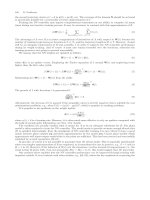
Starting from the above relationships and accounting for the calculations performed inside the network,
the general form of the NOE RNN can also be written as function of network weights
ˆy(t|θ)=f
⎛
⎝
nh

i=1
v
i
g
⎛
⎝
ni

j=1

w
ij
ϕ
j
(t)
⎞
⎠
⎞
⎠
, (9)
where nh is the number of nodes in the hidden layer and ni the number of input nodes, v
i
represents the
weight between the i-th node in the hidden layer and the output node, while w
ij
is the weight connecting the
j-th input node and the i-th node in the hidden layer. These weights are the components of the parameters
vector and ϕ
j
(t)isthej-th element of the input vector (8). The activation function g(.) in the hidden layer
nodes is the following non-linear sigmoid function:
g(x)=
2
1+exp(−2x + b)
− 1[−1; 1], (10)
where b is an adjustable bias term; at the output node the linear activation function f(.) is assumed.
Then, accounting for all the weights and biases the parameters vector is θ =[v
1
, v
nh

,w
11
, w
nh,ni
,
b
1
, b
nh
,b
no
].
4.1 Dynamic Network Features
Like the static MLPFF networks, RNN learning and generalization capabilities are the main features to be
considered during network development. The former deals with the ability of the learning algorithm to find the
set of weights which gives the desired accuracy, according to a criterion function. The generalization expresses
the neural network accuracy on a data set different from the training set. A satisfactory generalization can
be achieved when the training set contains enough information, and the network structure (i.e. number of
layers and nodes, feedback connections) has been properly designed. In this context, large networks should
be avoided because a high number of parameters can cause the overfitting of the training pattern through
an overparametrization; whilst under-sized networks are unable to learn from the training pattern; in both
cases a loss of generalization occurs. Furthermore, for a redundant network, the initial weights may affect the
learning process leading to different final performance, not to mention computational penalty. This problem
has not been completely overcome yet and some approaches are available in the literature: notably the works
of Atiya and Ji [8] and Sum et al. [46] give suggestions on the initial values of the network parameters. The
authors themselves have faced the problem of network weights uniqueness, making use of clustering methods
in the frame of a MonteCarlo parameters identification algorithm [34], in case of steady state networks.
Recurrent Neural Networks for AFR Estimation and Control in Spark Ignition Automotive Engines 151
Following recommendations provided by Thimm and Fiesler [48] and Nørgaard et al. [38], the weights are
initialized randomly in the range [−0.5 to 0.5] to operate the activation function described by (10) in its linear

region. Several studies have also focused on the definition of the proper network size and structure through
the implementation of pruning and regularization algorithms. These techniques rearrange the connection
levels or remove the redundant nodes and weights as function of their marginal contribution to the network
precision gained during consecutive training phases [17, 43]. For Fully Recurrent Neural Networks the issue of
finding the network topology becomes more complex because of the interconnections among parallel nodes.
Thus, specific pruning methodologies, such as constructive learning approach, have been proposed in the
literature [15, 28].
Some approaches have been followed to improve the network generalization through the implementation
of Active Learning (AL) Techniques [3]. These methods, that are derived from the Experimental Design
Techniques (EDT), allow reducing the experimental effort and increase the information content of the training
data set, thus improving the generalization. For static MLPFF networks the application of information-based
techniques for active data selection [14, 29] addresses the appropriate choice of the experimental data set
to be used for model identification by an iterative selection of the most informative data. In the field of
Internal Combustion Engine (ICE), these techniques search in the independent variables domain (i.e. the
engine operating conditions) for those experimental input–output data that maximize system knowledge [3].
Heuristic rules may be followed to populate the learning data set if AL techniques are awkward to
implement. In such a case, the training data set must be composed of experimental data that span the whole
operating domain, to guarantee steady-state mapping. Furthermore, in order to account for the dynamic
features of the system, the input data must be arranged in a time sequence which contains all the frequencies
and amplitudes associated with the system and in such a way that the key features of the dynamics to be
modeled will be excited [38]. As it will be shown in the following section, a pseudo-random sequence of input
data has been considered here to meet the proposed requirements.
The RNN described through the relationships (7) and (8) is a discrete time network, and a fixed sampling
frequency has to be considered. To build the time dependent input–output data set, the sampling frequency
should be high enough to guarantee that the dynamic behaviour of the system is well represented in the
input–output sequence. Nevertheless, as reported in Nørgaard et al. [38], the use of a large sampling frequency
may generate numerical problems (i.e. ill-conditioning); moreover, when the dimension of the data sequence
becomes too large an increase of the computational burden occurs.
A fundamental feature to be considered for dynamic modeling concerns with the stability of the solution.
RNNs behave like dynamic systems and their dynamics can be described through a set of equivalent nonlinear

Ordinary Differential Equations (ODEs). Hence, the time evolution of a RNN can exhibit a convergence to
a fixed point, periodic oscillations with constant or variable frequencies or a chaotic behavior [41]. In the
literature studies on stability of neural networks belong to the field of neurodynamics which provides the
mathematical framework to analyze their dynamic behavior [17].
4.2 Recurrent Neural Network Architectures for AFR Control
Neural Network based control systems are classified into two main types: (a) Direct Control Systems and
(b) Indirect Control Systems [38] as described in the following sections.
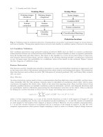
Direct Control System
In the Direct Control Systems (DCS) the neural network acts as a controller which processes the signals
coming from the real system. The control signals are evaluated as function of the target value of the controlled
variable. In this section two different DCS are presented: the Direct Inverse Model (DIM) and the Internal
Model Control (IMC). A description of these two approaches is given below.
Direct Inverse Model
The basic principle of this methodology is to train the Neural Network (i.e. identification of the Network
parameters) to simulate the “inverse” dynamics of the real process and then to use the inverse model as a
152 I. Arsie et al.
u(t)
FRQWURO
IRNNM
Plant
r(t+1)
y(t+1)
D
D
WDUJHW
RXWSXW
D
D
Fig. 4. Direct Inverse Model (DIM) based on a NOE network (Inverse RNNM). The control signal is estimated at
the time t as a function of the desired value r(t + 1) and the feedbacks. Note that the parameters m and n (see (12))

have been assumed equal to 2
controller. Assuming that the dynamics of the system can be described through an RNN model analogous
to the one proposed in (7) and (8)
ˆy(t +1)=F [ˆy(t), ,ˆy(t − n +1),x(t), ,x(t −m +1)]. (11)
For a generic MIMO the Inverse RNN Model (IRNNM) is obtained by isolating the most recent control
input as follows:
ˆu(t)=F
−1
[y(t +1),y(t), ,y(t −n +1), ,ˆu(t −1), ,ˆu(t − m +1)]. (12)
It is worth remarking that the u notation in (12) replaces “x” to highlight that in control applications all or
some external variables (depending on plant typology, e.g. SISO, MISO or MIMO) are control variables too.
Once the network has been trained, it can be used as a controller by substituting the output ˆy(t+ 1) with
the desired target value r(t + 1). Assuming that the model (12) describes accurately the inverse dynamics
of the system, the computed control signal ˆu will be able to drive the system output y(t + 1) to the desired
value r(t + 1). Figure 4 shows the block-diagram of a DIM. It is worth noting that the desired value r is at
the time t + 1 while the control input ˆu refers to the time t; hence the controller performs the control action
one time step earlier than the desired target.
The advantages of the DIM approach are the simple implementation and the Dead-Beat built-in control
properties (i.e. fast response for wide and sudden variations of the state variables) [38]. Nevertheless, since
the controller parameters are identified in off-line, the DIM does not perform as an adaptive control system.
In order to develop an adaptive system, on-line training methodologies are required. The suitability of the
inverse neural controllers to control complex dynamic processes is confirmed by several studies, particularly
in the field of aerospace control systems (e.g. Gili and Battipede [16]).
Internal Model Control
The IMC control structure is derived from the DIM, described in the previous section, where a Forward RNN
Model (FRNNM) of the system is added to work in parallel with an IRNNM. Figure 5 shows a block diagram
of this control architecture. The output values predicted by the FRNNM are fed back to the IRNNM, that
evaluates the control actions as function of the desired output at the next time step r(t +1).Themore the
FRNNM prediction is accurate, the less the difference between FRNNM and Plant outputs will be. However,
the differences between Plant and FRNNM may be used to update the networks on-line (i.e. both IRNNM

and FRNNM), thus providing the neural controller with adaptive features.
The stability of the IMC scheme (i.e. the closed-loop system and the compensation for constant noises)
is guaranteed if both the real system and the controller are stable [22]. Despite their stringent requirements,
the IMC approach seems to be really appealing, as shown by several applications in the field of chemical
processes control (e.g. Hussain [23]).
Recurrent Neural Networks for AFR Estimation and Control in Spark Ignition Automotive Engines 153
System
y(t+1)
NN ControllerFilter
NN Forward
Model
û(t)
r(t+1)
-
+
-
D
D
D
+
System
y(t+1)
NN ControllerFilter
NN Forward
Model
û(t)
r(t+1)
-
+
-

D
D
D
+
Fig. 5. Neural Networks based Internal Model Control Structure (dashed lines – closed loop connections)
Indirect Control Systems
Following the classification proposed by Nørgaard et al. [38], a NN based control structure is indirect if the
control signal is determined by processing the information provided from both the real system and the NN
model. The Model Predictive Control (MPC) structure is an example of such control scheme.
Model Predictive Control
The MPC computes the optimal control signals through the minimization of an assigned Cost Function (CF).
Thus, in order to optimize the future control actions, the system performance is predicted by a model of the
real system. This technique is suitable for those applications where the relationships between performances,
operating constraints and states of the system are strongly nonlinear [23]. In the MPCs the use of the
Recurrent Neural Networks is particularly appropriate because of their nonlinear mapping capabilities and
dynamic features.
In the MPC scheme, a minimization of the error between the model output and the target values is
performed [38]. The time interval on which the performance are optimized starts from the current time t to
the time t + k. The minimization algorithm accounts also for the control signals sequence through a penalty
factor ρ. Thus, the Cost Function is
J(t, u(t)) =
N
2

i=N
1
[r(t + i) − ˆy(t + i)] + ρ
N
3


i=1
[∆u(t + i − 1)]
2
, (14)
where the interval [N
1
,N
2
] denotes the prediction horizon, N
3
is the control horizon, r is the target value of
the controlled variable, ˆy is the model output (i.e. the NN) and ∆u(t + i − 1) are the changes in the control
sequences.
In the literature, several examples dealing with the implementation of the MPCs have been proposed.
Manzie et al. [32] have developed a MPC based on Radial Basis Neural Networks for the AFR control.
Furthermore, Hussain [23] reports the benefits achievable through the implementation of NN predictive
models for control of chemical processes.
5 Model Identification
This section deals with practical issues associated with Recurrent Networks design and identification, such
as choice of the most suitable learning approach, selection of independent variables (i.e. network external
input x) and output feedbacks, search of optimal network size and definition of methods to assess RNN
generalization.
154 I. Arsie et al.
5.1 RNN Learning Approach
The parameters identification of a Neural Network is performed through a learning process during which a
set of training examples (experimental data) is presented to the network to settle the levels of the connections
between the nodes. The most common approach is the error Backpropagation algorithm due to its easy-to-
handle implementation. At each iteration the error between the experimental data and the corresponding
estimated value is propagated backward from the output to the input layer through the hidden layers. The
learning process is stopped when the following cost function (MSE) reaches its minimum:

E(θ)=
1
2N
N

t=1
(ˆy(t|θ) − y(t))
2
. (15)
N is the time horizon on which the training pattern has been gathered from experiments. The Mean
Squared Error (MSE) (15) evaluates how close is the simulated pattern ˆy(t|θ)[t =1,N] to the training
y(t)[t =1,N]. The Backpropagation method is a first-order technique and its use for complex networks might
cause long training and in some cases a loss of effectiveness of the procedure. In the current work, a second-
order method based on the Levenberg–Marquardt optimization algorithm is employed [17, 18, 38, 41, 43].
To mitigate overfitting, a regularization term [38] has been added to (15), yielding the following new cost
function:
E
∗
(θ)=
1
2N
N

t=1
(ˆy(t|θ) − y(t))
2
+
1
2N
· θ

T
· α ·θ, (16)
where α is the weight decay.
The above function minimization can be carried out in either a batch or pattern-by-pattern way. The
former is usually preferred at the initial development stage, whereas the latter is usually employed in on-line
RNN implementation, as it allows to adapt network weights in response to the exogenous variations of the
controlled/simulated system.
The training process aims at determining RNN models with a satisfactory compromise between precision
(i.e. small error on the training-set) and generalization (i.e. small error on the test-set). High generalization
cannot be guaranteed if the training data-set is not sufficiently rich. This is an issue of particular relevance
for dynamic networks such as RNN, since they require the training-set not only to cover most of the system
operating domain, but also to provide accurate knowledge of its dynamic behavior. Thus, the input data
should include all system frequencies and amplitudes and must be arranged in such a way that the key
features of the dynamics to be modeled are excited [38]. As far as network structure and learning approach
are concerned, the precision and generalization goals are often in conflict. The loss of generalization due
to parameters redundancy in model structure is known in the literature as overfitting [37]. This latter may
occur in the case of a large number of weights, which in principle improves RNN precision but may cause
generalization to decrease. A similar effect can occur if network training is stopped after too many epochs.
Although this can be beneficial to precision it may negatively impacts generalization capabilities and is known
as overtraining. Based on the above observations and to ensure a proper design of RNNs, the following steps
should be taken:
1. Generate a training data set extensive enough to guarantee acceptable generalization of the knowledge
retained in the training examples
2. Select the proper stopping criteria to prevent overtraining
3. Define the network structure with the minimum number of weights
As far as the impact of point (1) on the current application, AFR dynamics can be learned well by
the RNN estimator once the trajectories of engine state variables (i.e. manifold pressure and engine speed)
described in the training set are informative enough. This means that the training experiments on the test-
bench should be performed in such a way to cover most of the engine working domain. Furthermore a proper
description of both low- and high-frequency dynamics is necessary, thus the experimental profile should be

obtained by alternating steady operations of the engine with both smooth and sharp acceleration/deceleration
maneuvers.
Recurrent Neural Networks for AFR Estimation and Control in Spark Ignition Automotive Engines 155
Point (2) is usually addressed by employing the early stopping method. This technique consists of inter-
rupting the training process, once the MSE computed on a data set different from the training one stops
decreasing. Therefore, when the early stopping is used, network training and test require at least three data
sets [17]: training-set (set A), early stopping test-set (set B) and generalization test-set (set C).
Finally, point (3) is addressed by referring to a previous paper [6], in which a trial-and-error analysis
was performed to select the optimal network architecture in terms of hidden nodes and lag space. Although
various approaches on choosing MLPFF network sizing are proposed in the specific literature, finding the best
architecture for recurrent neural network is a challenging task due to the presence of feedback connections and
(sometimes) past input values [38]. In the current work the trial-and-error approach is used to address (3).
5.2 Input Variables and RNNs Formulation
Based on experimental tests, the instantaneous port air mass flow is known to be mainly dependent on
both manifold pressure and engine speed (i.e. engine state variables) [21]. On the other hand, the actual
fuel flow rate results from the dynamic processes occurring into the inlet manifold (see Fig. 1 and (1), (2)),
therefore the manifold can be studied as a Multi Input Single Output (MISO) system. In case of FRNNM
for AFR prediction, the output, control and external input variables are ˆy = AFR, u = t
inj
,x=[rpm, p
m
],
respectively and the formulation resulting from (7) and (8) will be
A
ˆ
FR(t, θ)=F [A
ˆ
FR(t −1|θ
1
), ,A

ˆ
FR(t −n|θ
1
),t
inj
(t − 1), ,t
inj
(t − m),
rpm(t −1), ,rpm(t − m),p
m
(t − 1), ,p
m
(t − m)].
(17)
It is worth noting that the output feedback in the regressors vector (i.e. A
ˆ
FR in (17)) is simulated by
the network itself, thus the FRNNM does not require any AFR measurement as feedback to perform the
on-line estimation. Though such a choice could reduce network accuracy [38], it allows to properly address
the AFR measurement delay issue due to mass transport, exhaust gas mixing and lambda sensor response
[39]. This NOE feature is also very appealing because it enables AFR virtual sensing even when the oxygen
sensor does not supply a sufficiently accurate measurement, as it happens during cold start phases.
Regarding AFR control, a DIM structure (see Fig. 4) is considered for the current application. Hence the
IRNNM can be obtained by inverting (7), yielding the following RNN expression:
ˆ
t
inj
(t − 1|θ
2
)=G[A

ˆ
FR(t|θ
1
), ,A
ˆ
FR(t − n|θ
1
),
ˆ
t
inj
(t − 2|θ
2
), ,
ˆ
t
inj
(t − m|θ
2
)
rpm(t −1), ,rpm(t −m),p
m
(t − 1), ,p
m
(t − m)],
(18)
where A
ˆ
FR is the estimate provided by FRNNM and θ
2

is the IRNNM parameters vector.
Afterwards, substituting A
ˆ
FR(t +1|θ
1
) by the future target value AF R
des
, the control action can be
computed as
ˆ
t
inj
(t − 1|θ
2
)=G[AF R
des
(t), ,A
ˆ
FR(t −n|θ
1
),
ˆ
t
inj
(t − 2|θ
2
), ,
ˆ
t
inj

(t − m|θ
2
)
rpm(t −1), ,rpm(t −m),p
m
(t − 1), ,p
m
(t − m)].
(19)
6 Experimental Set-Up
The RNN AFR estimator and controller were trained and tested vs. transient data sets measured on the
engine test bench at the University of Salerno. The experiments were carried out on a commercial engine,
four cylinders, 1.2 liters, with Multi-Point injection. It is worth noting that due to the absence of a camshaft
sensor, the injection is not synchronized with the intake stroke, therefore it takes place twice a cycle for
each cylinder. The test bench is equipped with a Borghi & Saveri FE-200S eddy current dynamometer. A
data acquisition system, based on National Instruments cards PCI MIO 16E-1 and Sample & Hold Amplifier
SC-2040, is used to measure engine variables with a sampling frequency up to 10 kHz. An AVL gravimetric
balance is used to measure fuel consumption in steady-state conditions to calibrate the injector flow rate.
156 I. Arsie et al.
Engine
AVL-Puma
rpm
Micro
Autobox
P
m
, rpm
t
inj
, θ

s
Dyno
β
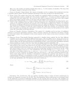
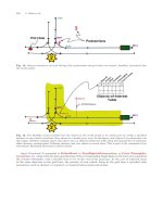
Fig. 6. Lay-out of the experimental plant. β = throttle opening, θ
s
= spark advance, t
inj
= injection time
Fig. 7. Location of the UEGO sensor (dotted oval)
The engine control system is replaced with a dSPACE
c
 MicroAutobox equipment and a power conditioning
unit. Such a system allows to control all the engine tasks and to customize the control laws. To guarantee
the controllability and reproducibility of the transient maneuvers, both throttle valve and engine speed are
controlled through an AVL PUMA engine automation tool (see Fig. 6).
The exhaust AFR is sensed by an ETAS Lambda Meter LA4, equipped with a Bosch LSU 4.2 UEGO
sensor. This is placed right after the exhaust valve of the first cylinder (see Fig. 7) to investigate the air–
fuel mixing process in one cylinder only. This choice allows to remove the dynamic effects induced by gas
transport and mixing phenomena occurring in the exhaust pipes. Also non predictable effects generated by
cylinder-to-cylinder unbalance due to uneven processes such as air breathing, thermal state and fuel injection
can be neglected. Therefore, the time shift between injection timing and oxygen sensor measurement mostly
accounts for pure engine cycle and lack of synchronization between injection and intake valve timing. This
latter term can be neglected in case of synchronized injection. As mentioned before, the time delay could
represent a significant problem for control applications [10, 24, 32, 42] and the accomplishment of this task
isdescribedinSect.6.1.
6.1 Training and Test Data
The training and test sets were generated by running the engine on the test bench in transient conditions. In
order to span most of the engine operating region, perturbations on throttle and load torque were imposed
during the transients. Fast throttle actions, with large opening-closing profiles and variable engine speed
set points, were generated off-line and assigned through the bench controller to the engine and the dyno,

respectively (see Fig. 6). Regarding fuel injection, only the base injection task (see Fig. 2) was executed,
thus allowing to investigate the dynamic behavior of the uncontrolled plant, without being affected by
neither feedforward nor feedback compensation. Furthermore, in order to excite the wall wetting process
Recurrent Neural Networks for AFR Estimation and Control in Spark Ignition Automotive Engines 157
Fig. 8. Training data set (SET A)
independently from the air breathing dynamics, a uniform random perturbation was added to the injection
base time, limiting the gain in the range ±15% of the nominal fuel injection time (i.e. duration of time when
the injector is open). Such an approach protects the RNN from unacceptable accuracy of predictions in the
case of injection time deviation at constant engine load and speed as it is the case when a different AFR
target is imposed. This matter is extensively described in our previous work [6].
In Fig. 8 the measured signals of throttle opening (a), engine speed (b), manifold pressure (c), injection
time (d) and AFR (e) used as training-data (Set A) are shown. The throttle opening transient shown in
Fig. 8a allows exciting the filling-emptying dynamics of the intake manifold and the engine speed dynamics,
as a consequence of both engine breathing and energy balance between engine and load torque. Fig. 8b, c
indicate that the transient spans most of the engine operating domain with engine speed and manifold
pressure ranging from 1,000 to 4,000 rpm and from low to high load, respectively. The variation of manifold
pressure and engine speed affects the intake air flow rate and consequently the amount of fuel to be injected
to meet the target AFR. It is worth noting that the manifold pressure signal was filtered in order to cancel
the process noise that has negligible effects on the AFR dynamic response. This enhances the FRNNM
in learning the main manifold dynamics without being perturbed by second order phenomena (e.g. intake
manifold pressure fluctuation).
158 I. Arsie et al.
Fig. 9. Test data set (SET B)
The injection time trajectory (Fig. 8d), commanded by the ECS, excites the wall wetting dynamics,
which in turn influences the in-cylinder AFR in a broad frequency range. It is also worth to mention that
engine speed and throttle opening are decoupled to generate more realistic engine speed–pressure transients.
Furthermore, the speed dynamics is more critical as compared to what occur on a real vehicle, due to the
lower inertia of the engine test-bench.
Figure 9 shows the time histories of throttle opening, engine speed, manifold pressure and injected fuel
measured for the test-set (SET B). SET B was obtained imposing square wave throttle maneuvers (Fig. 9a)

to excite the highest frequencies of the air dynamics, while keeping the engine speed constant (Fig. 9b)
and removing the fuel pulse random perturbation. Figure 9d, e evidence that the resulting step variations of
injected fuel generate wide lean/rich spikes of AFR, due to uncompensated effects of wall wetting dynamics
during abrupt throttle opening/closing transients. Such features make SET B suitable as test data-set since
RNN accuracy in predicting high frequency dynamic response is demanded. Moreover, the step variations
of injected fuel are also appropriate to estimate the AFR delay. Thus, SET B is also very suitable to assess
the ability of RNN to cope with the pure time delay.
Recurrent Neural Networks for AFR Estimation and Control in Spark Ignition Automotive Engines 159
It is worth noting that the early stopping was not applied directly, in that the maximum number of
training epochs was set to 50 following recommendations from the previous study where an early stopping
data set was used [7].
FRNNM: AFR Prediction
The identification task of the FRNMM was performed on a NOE structure consisting of 12 hidden nodes,
with lag spaces n = 2 and m = 5 (see (17)) [6]. SET A was used to train the RNN with a number of training
epochs set to 50. This value was selected according to the results shown in the previous work [7] where the
early stopping criterion was utilized to maximize RNN generalization. The training procedure was applied
four times to investigate the influence of the time delay ∆t
AF R
between AFR measurement and triggering
signal (i.e. injection timing) on RNN accuracy. Table 1 lists the four cases analyzed, with the time delay
expressed as function of the engine speed (ω).
In Cases 2, 3 and 4, the AFR signal was back-shifted by the corresponding delay. Case 2 accounts for
the pure delay due to the engine cycle, that can be approximated as one and a half engine revolution, from
middle intake stroke to middle exhaust stroke (i.e. 3π/ω) as suggested by [39]. In Cases 3 and 4, instead,
the delay was assumed longer than 3π/ω, thus allowing to account for other delays that could occur. They
include injection actuation, lack of synchronization between injection and intake valve timing, unsteadiness
of gas flowing through the measuring section and mixing in the pipe with residual gas from the previous
cycle. The value assumed for the extreme Case 4 is in accordance with the delay proposed by Powell et al.
[42] for an oxygen sensor located in the main exhaust pipe after the junction. In this study, the delay in the
set-up of Fig. 6 can be determined by comparing the performance achieved by the RNN estimator on SET

A and SET B for the four delay scenarios. Figures 10 and 11 summarize the results of this comparison.
The general improvement in accuracy was expected due to the simpler dynamics resulting from delay
removal. In this way the RNN is not forced to learn the delay as part of the process dynamics, thus enhancing
Tab l e 1. Delay scenarios analyzed for RNN training
Case 1 Case 2 Case 3 Case 4
∆t
AFR
(s) 0 3π/ω 5π/ω 6π/ω
Fig. 10. Comparison between measured and predicted AFR in presence of rich excursions (SET B)
160 I. Arsie et al.
5 5.5 6 6.5 7 7.5 8
12
13
14
15
16
17
18
19
20
Time [s]
AFR [/]
measured
predicted
AFR [/] (Case 1)
5 5.5 6 6.5 7 7.5 8
12
13
14
15

16
17
18
19
20
Time [s]
AFR [/] - (Case 2)
5 5.5 6 6.5 7 7.5 8
12
13
14
15
16
17
18
19
20
Time [s]
AFR [/] (Case 3)
5 5.5 6 6.5 7 7.5 8
12
13
14
15
16
17
18
19
20
21

Time [s]
AFR [/] (Case 4)
5 5.5 6 6.5 7 7.5 8
12
13
14
15
16
17
18
19
20
Time [s]
AFR [/]
measured
predicted
AFR [/] (Case 1)
5 5.5 6 6.5 7 7.5 8
12
13
14
15
16
17
18
19
20
Time [s]
measured
predicted

5 5.5 6 6.5 7 7.5 8
12
13
14
15
16
17
18
19
20
Time [s]
AFR [/] - (Case 2)
5 5.5 6 6.5 7 7.5 8
12
13
14
15
16
17
18
19
20
Time [s]
AFR [/] (Case 3)
5 5.5 6 6.5 7 7.5 8
12
13
14
15
16

17
18
19
20
21
Time [s]
AFR [/] (Case 4)
AFR [/] (Case 1)
Fig. 11. Comparison between measured and predicted AFR in presence of lean excursions (SET B)
the training task. More specifically, the analysis of the errors indicates that the best result with respect to
SET B occurs for Case 3. Figures 10 and 11 show the comparison of AFR traces in both rich and lean
transients. In Fig. 10 it is evident how the Case 3 RNN performs the best estimation of the rich spike and,
moreover, simulates it with the correct dynamics. Figure 11 confirms this behavior for lean spike reproduction
as well.
The above observations led to select Case 3 as the best case and, as a consequence, the AFR trace was
back-shifted by a time delay corresponding to 5π/ω crank-shaft interval. The assumed time interval accounts
for the engine cycle delay (3π/ω) plus the effect due to the lack of synchronization between injection and
intake stroke; this latter can be approximated, in the average, with a delay of 2π/ω. Furthermore, the delay
of 5π/ω is also in accordance with the value proposed by Inagaki et al. [24] for similar engine configuration
and lambda sensor location.
IRNNM: Real-Time AFR Control
A DIM-based neural controller (see Fig. 4) was set-up to implement the AFR control law detailed above
(i.e. (19)). In this configuration, sketched in Fig. 12, the IRNNM is coupled to the FRNNM, which replaces
the plant in providing the AFR feedback to the IRNNM without measuring delay, as discussed in the previous
section. This FRNNM feature is particularly beneficial because it allows to simplify the IRNNM structure
[38], in that no delay has to be included in the corresponding regression vector. It is also worth remarking
that RNN structures can only include constant delay in the time domain, whereas the accounted AFR
measurement delay is mainly constant in the frequency domain, thus variable in the time domain [39].
Figure 12 also shows that the AFR values predicted by the FRNNM are fed as feedbacks to the IRNNM,
which evaluates the control actions as function of FRNNM feedbacks, desired AFR at next time step (t +1)

and current and past external variables provided by engine measurements (i.e. rpm (t −1,t−m),p
m
(t −1,
t −m)). The more accurate the FRNNM prediction is, the less the difference between FRNNM and Plant
outputs will be. However, the differences between Plant and FRNNM may be used to update the networks
on-line (i.e. both IRNNM and FRNNM), thus providing the neural controller with adaptive features.
According to the selected neural controller architecture, the IRNNM was trained by means of the iden-
tification procedure sketched in Fig. 13, on the same SET A assumed for the FRNNM training. Following
the formulation described in (18), the AFR fed to the network is nothing but the prediction performed by
Recurrent Neural Networks for AFR Estimation and Control in Spark Ignition Automotive Engines 161
IRNNM
FRNNM
D
)(
ˆ
tRFA
)(tAFR
()
1+tAFR
des
)1(
ˆ
−tt
inj
[
]
)(
ˆ
,),2(
ˆ

mtttt
inj
inj
−−
[]
)( ,),1( mtrpmtrpm −−
[]
)( ,),1( mtptp
mm
−−
)(trpm
)(tp
m
[
]
)(
ˆ
,),1(
ˆ
ntRFAtRFA −−
D
Plant
(SI Engine)
D
D
-
-
Fig. 12. DIM neural controller based on the integration of DIM and FRNNM. The control signal t
inj
is estimated

as function of the desired AFR value at time t + 1, the feedbacks from both IRNNM and FRNNM and the external
variable values provided by plant measurements. Note that the dashed lines in the IRNNM box mean that the
corresponding inputs are passed to the FRNNM too
Fig. 13. Training structure adopted for the IRNNM. Note that feedback connections are omitted for simplicity
the FRNNM, while engine speed and manifold pressure values correspond to the measured signals shown
in Fig. 8 [set A]. The training algorithm was then aimed at minimizing the residual between simulated and
experimental injected fuel time histories.
A preliminary test on the inverse model was accomplished off-line by comparing simulated and
experimental injected fuel signals in case of data sets A and B.
162 I. Arsie et al.
Afterwards, a real-time application was carried out by implementing the neural controller architec-
ture (see Fig. 12) in the engine control system on the test bench. The neural controller was employed in
Matlab
c
/Simulink environment and then uploaded to the dSPACE
c
 MicroAutobox equipment. Accord-
ing to the formulation presented in (19), the controller is intended to provide the actual injection time by
processing actual and earlier measurements of engine speed and manifold pressure, and earlier prediction of
AFR performed by the FRNMM. Furthermore, unlike the preliminary test, the target AFR has also to be
imposed and it was set to the stoichiometric value for the current application.
As mentioned above, due to the UEGO sensor location, the controller was tested on the first cylinder only,
while the nominal map based injection strategy was used for the three remaining cylinders. The results of
the controller performance in tracking the target AFR along the engine test transient (SET B) are discussed
in the next section.
7Results
As described in the previous section, the training SET A has been used to design the RNNs that simulate
both forward and inverse dynamics of the fuel film in the intake manifold. The test transient SET B has
been simulated to verify the network generalization features. Furthermore, on-line implementation of the
two networks was carried out to test, again on SET B, the performance of the neural controller (see Fig. 12)

proposed in this work to limit AFR excursions from stoichiometry.
7.1 FRNNM: AFR Prediction
The accuracy of the developed FRNNM is demonstrated by the small discrepancies between measured and
predicted AFR, as shown in detail in Figs. 14, 15, 16 and 17 for both SET A and SET B. Particularly,
Figs. 16 and 17, which refer to abrupt throttle opening/closing maneuvers (see Fig. 9a), show that the delay
removal from the AFR signal enables the FRNNM to capture AFR dynamics in both rich and lean transients
very well [7]. Figures 16 and 17 also indicate how the simulated AFR trajectory is smoother as compared to
the more wavy experimental profile.
This behavior is due to the pressure signal filtering, mentioned in Sect. 6.1, and confirms that this pro-
cedure allows retaining suitable accuracy in predicting AFR dynamic response during engine transients.
Particularly, Fig. 14 shows that the FRNNM correctly follows small-amplitude AFR oscillations when sim-
ulating the training transient (SET A), thus indicating that the signal filtering does not affect FRNNM
accuracy in predicting AFR dynamics.
Fig. 14. Trajectories of measured and predicted AFR (SET A, time window [50–60])
Recurrent Neural Networks for AFR Estimation and Control in Spark Ignition Automotive Engines 163
Fig. 15. Trajectories of measured and predicted AFR (SET B)
Fig. 16. Trajectories of measured and predicted AFR (SET B, time window [5, 8])
Fig. 17. Trajectories of measured and predicted AFR (SET B, time window [37, 41])
It is worth noting that the inaccurate overshoot predicted by the FRNMM (see Fig. 15 at 20 s and
45 s) is due to the occurrence of a dramatic engine speed drop induced by a tip-out maneuver, resulting in
the pressure increase shown on Fig. 9c. This experimental behavior is explained considering that the test
dynamometer is unable to guarantee a constant engine speed when an abrupt throttle closing is imposed
164 I. Arsie et al.
at medium engine speed and low loads (i.e. 2,500 rpm, from 25
◦
to 15
◦
). Actually, in such conditions, the
dynamometer response is not as fast as it should be in counterbalancing the engine torque drop and an over-
resistant torque is applied to the engine shaft. It is worth mentioning that such transient is quite unusual

with respect to the in-vehicle engine operation.
7.2 IRNNM: AFR Control
As explained in Sect. 6.1, the IRNNM was trained by feeding as input the AFR predicted by the virtual
sensor (i.e. FRNNM). The RNN structure adopted to simulate inverse AFR dynamics was obtained through
the inversion of the FRNNM structure (i.e. 12 hidden nodes, n = 2, m = 5), according to the modeling
scheme discussed above (see (18)).
Figure 18 shows the comparison between IRNNM and experimental injection time for the entire SET
B. The trained IRNNM approximates the inverse AFR dynamics as accurately as the FRNNM does for the
forward dynamics. Regarding the more wavy profile simulated by the IRNNM, it can be explained considering
that this network was trained on t
inj
profile from Fig. 9 heavily perturbed by the noise as mentioned in
Sect. 6.1. Therefore, it tends to amplify the AFR oscillations in SET B (see Fig. 9e), although they are of
smaller amplitude as compared to the ones measured in the training transient (see Fig. 8). Nevertheless, this
effect is well balanced by the benefits provided by the random t
inj
perturbation, both in terms of IRNNM
generalization [6] and direct controller performance, as discussed below.
Online tests of the developed RNNs were performed by integrating the FRNNM and IRNNM in the
framework of a dSPACE
c
 MicroAutobox control unit for the adopted neural controller (see Fig. 12). The
experiments were conducted reproducing, by means of the automated test bench controller, the same transient
used as test-set (i.e. SET B), this time evaluating the injection time with the neural controller. The target
value of AFR to be fed to the IRNNM (i.e. (19)), was set to stoichiometry, i.e. 14.67. In order to assess
the performance of the proposed controller thoroughly, the resulting AFR trajectory was compared to the
trajectory measured from the actions of the reference ECU (see Fig. 2), as shown in Figs. 19 and 20. The
lines corresponding to AFR
des
=14.67, AFR

des
+5%and AFR
des
− 5% are also plotted in the figures.
Figure 19 shows how the performance level achieved by the two controllers is very close. It is interesting
to note how the neural controller performs better (maneuvers 3rd, 5th, 7th) or worse (maneuvers 1st, 4th,
8th) than the ECU in limiting AFR spikes when abrupt throttle opening/closing are performed (see Fig. 9a).
Particularly, in Fig. 20 it can be seen how the feedback action performed by the neural controller on the
AFR predicted by the virtual sensor induces a higher-order AFR response as compared to that obtained
with ECU. This results in a faster AFR compensation (0.5 s against 1 s) and, particularly, in removing the
Fig. 18. Trajectories of measured and predicted injection time (SET B)
Recurrent Neural Networks for AFR Estimation and Control in Spark Ignition Automotive Engines 165
Fig. 19. Comparison between reference ECU and our NN performance in terms of AFR control (SET B)
Fig. 20. Comparison between reference ECU and our NN performance in terms of AFR control (SET B, time window
[40, 44] of Fig. 19)
AFR overshoot observed with the ECU. Of course, neither the neural controller nor the ECU can overcome
the rich excursion due to the fuel puddle on manifold walls, unless a suitable strategy aimed at increasing the
air flow rate is actuated. Our result demonstrate a potential of Neural Networks in improving current AFR
control strategies with a significant reduction of experimental burden and calibration effort with respect to
conventional approaches.
8Conclusion
Recurrent Neural Network models have been developed to simulate both forward and inverse air–fuel ratio
(AFR) dynamics in an SI engine. The main features of RNNs have been reviewed with emphasis on obtaining
reliable models with high degree of generalization for practical engine applications.
Training and test data sets have been derived from experimental measurements on the engine test bench
by imposing load and speed perturbations. To enhance RNN generalization, the input variables have been
uncorrelated by perturbing the fuel injection time around the base stoichiometric amount. Moreover, the
removal of a 5π/ω delay from the measured AFR signal was proven to be necessary to ensure accurate
prediction of AFR dynamics for both rich and lean transients.
166 I. Arsie et al.

The virtual sensor (i.e. FRNNM) has shown satisfactory prediction of the AFR dynamics with an esti-
mation error over the measured trajectory lower than 2% for most of the test transients, even in the presence
of wide AFR spikes, thus proving that the RNN dynamic behavior is satisfactorily close to the real system
dynamics.
A real-time application of the direct AFR neural controller based on the inverse model (i.e. IRNNM) has
been accomplished. The controller that also makes use of the virtual sensor prediction has been implemented
on the engine control unit and tested over experimental transients. The comparison with the AFR trajectory
resulting from the action of the reference ECU provides evidence of a good performance of the controller.
Specifically, the integration with the virtual sensor prediction induces a higher-order response that results
in faster AFR compensation and, especially, in reducing overshoots observed with the reference ECU con-
trol strategy. The results demonstrate the potential offered by neural controllers to improve engine control
strategies, particularly considering the significant reduction of experimental burden/calibration efforts vs.
standard methodologies. The proposed neural controller is based on an open-loop scheme, therefore adap-
tive features can be introduced further by an on-line training aimed at adjusting IRNNM and FRNNM
parameters according to engine aging and/or faults.
References
1. Alippi C, de Russis C, Piuri V (2003) Observer-based air–fuel ratio control. IEEE Transactions on Systems, Man,
and Cybernetics – Part C: Applications and Reviews 33: 259–268.
2. Aquino CF (1981) Transient A/F control characteristics of the 5 liter central fuel injection engine. SAE paper
810494. SAE International, Warrendale.
3. Arsie I, Marotta F, Pianese C, Rizzo G (2001) Information based selection of neural networks training data for
S.I. engine mapping. SAE 2001 Transactions – Journal of Engines 110–3: 549–560.
4. Arsie I, Pianese C, Rizzo G, Cioffi V (2003) An adaptive estimator of fuel film dynamics in the intake port of a
spark ignition engine. Control Engineering Practice 11: 303–309.
5. Arsie I, Pianese C, Sorrentino M (2004) Nonlinear recurrent neural networks for air fuel ratio control in SI engines.
SAE paper 2004-01-1364. SAE International, Warrendale.
6. Arsie I, Pianese C, Sorrentino M (2006) A procedure to enhance identification of recurrent neural networks for
simulating air–fuel ratio dynamics in SI engines. Engineering Applications of Artificial Intelligence 19: 65–77.
7. Arsie I, Pianese C, Sorrentino M (2007) A neural network air–fuel ratio estimator for control and diagnostics
in spark-ignited engines. In: Fifth IFAC Symposium on Advances in Automotive Control, Monterey, CA, USA,

August 20–22, 2007.
8. Atiya A, Ji C (1997) How initial conditions affect generalization performance in large networks. IEEE Transactions
on Neural Networks 8: 448–454.
9. Capriglione D, Liguori C, Pianese C, Pietrosanto A (2003) On-line sensor fault detection isolation, and
accommodation in automotive engines. IEEE Transactions on Instrumentation and Measurement 52: 1182–1189.
10. Choi SB, Hedrick JK (1998) An observer-based controller design method for improving air/fuel characteristics
of spark ignition engines. IEEE Transactions on Control Systems Technology 6: 325–334.
11. Dinca L, Aldemir T, Rizzoni G (1999) A model-based probabilistic approach for fault detection and identification
with application to the diagnosis of automotive engines. IEEE Transactions on Automatic Control 44: 2200–2205.
12. Dovifaaz X, Ouladsine M, Rachid A (1999) Optimal control of a turbocharged diesel engine using neural network.
In: 14th IFAC World Congress, IFAC-8b-009, Beijing, China, July 5–9, 1999.
13. Fiengo G, Cook JA, Grizzle JW (2002) Fore-aft oxygen storage control. In: American Control Conference,
Anchorage, AK, May 8–10.
14. Fukumizu K (2000) Statistical active learning in multilayer perceptrons. IEEE Transactions on Neural Network
11: 17–26.
15. Giles CL, Chen D, Sun GZ, Chen HH, Lee YC, Goudreau MW (1995) Constructive learning of recurrent neu-
ral networks limitations of recurrent cascade correlation and a simple solution. IEEE Transactions on Neural
Networks 6: 829–835.
16. Gili PA, Battipede M (2001) Adaptive neurocontroller for a nonlinear combat aircraft model. Journal of Guidance,
Control and Dynamics 24(5): 910–917.
17. Haykin S (1999) Neural Networks. A Comprehensive Foundation, 2nd edn, Prentice-Hall, Englewood Cliffs, NJ.
18. Hecht-Nielsen R (1987) Neurocomputing. Addison-Wesley, Reading, MA.
Recurrent Neural Networks for AFR Estimation and Control in Spark Ignition Automotive Engines 167
19. Heimann B, Bouzid N, Trabelsi A (2006) Road–wheel interaction in vehicles a mechatronic view of friction. In:
Proceedings of the 2006 IEEE International Conference on Mechatronics, pp. 137–143, July 3–5, 2006.
20. Hendricks E, Sorenson SC (1991) SI engine controls and mean value engine modeling. SAE Paper 910258. SAE
International, Warrendale.
21. Heywood JB (1988) Internal Combustion Engine Fundamental. McGraw-Hill, New York.
22. Hunt KJ, Sbarbaro D (1991) Neural networks for nonlinear internal model control. IEEE proceedings D 138(5):
431–438.

23. Hussain MA (1999) Review of the applications of neural networks in chemical process control simulation and
online implementation. Artificial Intelligence in Engineering 13: 55–68.
24. Inagaki H, Ohata A, Inoue T (1990) An adaptive fuel injection control with internal model in automotive engines.
In: IECON ’90, 16th Annual Conference of IEEE, pp. 78–83.
25. Isermann R (1997) Supervision, fault-detection and fault-diagnosis methods – an introduction. Control
Engineering Practice 5: 638–652.
26. Kainz JL, Smith JC (1999) Individual cylinder fuel control with a switching oxygen sensor. SAE Paper 1999-01-
0546. SAE International, Warrendale.
27. Kim YW, Rizzoni G, Utkin V (1998) Automotive engine diagnosis and control via nonlinear estimation. IEEE
Control Systems Magazine 18: 84–99.
28. Lehtokangas M (1999) Constructive backpropagation for recurrent networks. Neural Processing Letters 9: 271–
278.
29. MacKay DJC (1992) Information-based objective functions for active data selection. Neural Computation
4: 590–604.
30. Malaczynski GW, Baker ME (2003) Real-time digital signal processing of ionization current for engine diagnostic
and control. SAE Paper 2003-01-1119, SAE 2003 World Congress & Exhibition, Detroit, MI, USA, March 2003.
31. Maloney PJ (2001) A production wide-range AFR – response diagnostic algorithm for direct-injection gasoline
application. SAE Paper 2001-01-0558, 2001. SAE International, Warrendale.
32. Manzie C, Palaniswami M, Ralph D, Watson H, Yi X (2002) Observer model predictive control of a fuel injection
system with a radial basis function network observer. ASME Journal of Dynamic Systems, Measurement, and
Control 124: 648–658.
33. Marko KA, James J, Dosdall J, Murphy J (1989) Automotive control system diagnostics using neural nets
for rapid pattern classification of large data sets. In: Proceedings of International Joint Conference on Neural
Networks, 1989 IJCNN, pp. 13–16, vol. 2, Washington, DC, July 18, 1989.
34. Mastroberti M, Pianese C (2001) Identificazione e Validazione diModelli a Rete Neurale per Motori ad Accensione
Comandata Mediante Tecniche Monte Carlo. In: 56th National Congress of ATI, Napoli, September 10–14 (in
italian).
35. Matthews RD, Dongre SK, Beaman JJ (1991) Intake and ECM sub-model improvements for dynamic SI engine
models: examination of tip-in tip-out. SAE Paper No. 910074. SAE International, Warrendale.
36. Nakae M, Tsuruta T, Mori R, Shinsuke I (2002) “Development of Planar Air Fuel Ratio Sensor”, SAE Paper

2002-01-0474.
37. Nelles O (2000) Nonlinear System Identification. Springer, Berlin.
38. Nørgaard M, Ravn O, Poulsen NL, Hansen LK (2000) Neural Networks for Modelling and Control of Dynamic
Systems. Springer, London.
39. Onder CH, Geering HP (1997) Model identification for the A/F path of an SI Engine. SAE Paper No. 970612.
SAE International, Warrendale.
40. Ortmann S, Glesner M, Rychetsky M, Tubetti P, Morra G (1998) Engine knock estimation using neural networks
based on a real-world database. SAE Paper 980513. SAE International, Warrendale.
41. Patterson DW (1995) Artificial Neural Networks – Theory and Applications. Prentice Hall, Englewood Cliffs, NJ.
42. Powell JD, Fekete NP Chang CF (1998) Observer-based air–fuel ratio control. IEEE Transactions on Control
Systems 18: 72–83.
43. Ripley BD (2000) Pattern Recognition and Neural Networks. Cambridge University Press, Cambridge.
44. Shayler PJ, Goodman MS, Ma T (1996) Transient air/fuel ratio control of an S.I. engine using neural networks.
SAE Paper 960326. SAE International, Warrendale.
45. St-Pierre M, Gingras D (2004) Neural network-based data fusion for vehicle positioning in land navigation system.
SAE Paper 2004-01-0752, SAE 2004 World Congress & Exhibition, Detroit, MI, USA, March 2004.
46. Sum J, Leung C, Young GH, Kann W (1999) On the Kalman filtering method in neural-network training and
pruning. IEEE Transactions on Neural Networks 10(1).
168 I. Arsie et al.
47. Tan Y, Saif M (2000) Neural-networks-based nonlinear dynamic modeling for automotive engines. Neurocomput-
ing 30: 129–142.
48. Thimm G, Fiesler E (1997) Higher order and multilayer perceptron initialization. IEEE Transaction Neural
Network 8: 349–359.
49. Turin RC, Geering HP (1994) Model-based adaptive fuel control in an SI engine. SAE Paper 940374. SAE
International, Warrendale.
50. Vigild CW, Andersen KPH, Hendricks E (1999) Towards robust H-infinity control of an SI engine’s air/fuel ratio.
SAE Paper 1999-01-0854. SAE International, Warrendale.
51. Yasuri Y, Shusuke A, Ueno M, Yoshihisa I (2000) Secondary O
2
feedback using prediction and identification type

sliding mode control. SAE Paper no. 2000-01-0936. SAE International, Warrendale.
52. Yoo IK, Upadhyay D, Rizzoni G (1999) A control-oriented carbon canister model. SAE Paper 1999-01-1103. SAE
International, Warrendale.