[Psychology] Mechanical Assemblies Phần 5 pptx
Bạn đang xem bản rút gọn của tài liệu. Xem và tải ngay bản đầy đủ của tài liệu tại đây (5.68 MB, 58 trang )
212
8 THE
DATUM FLOW CHAIN
FIGURE
8-1.
The
Stapler,
Its
Liaison Diagram
(left),
and Two Key
Characteristics
(right).
Several irrelevant liaisons
have
been
colored
gray because they play
no
role
in
positioning
parts
to
deliver
either
KC.
FIGURE
8-2.
The KCs of the
Stapler Shown Separately with
the
Liaisons
That Deliver Them. Irrelevant liaisons
are not
shown.
the
process
for
creating
it and
thus only indirectly
defines
the
assembly.
We
will
also
define
two
types
of
assembly joints,
called
mates
and
contacts: Mates pass dimensional constraint
from
part
to
part, while contacts merely provide support,
reinforcement,
or
partial constraint along axes that
do not
involve
delivery
of a KC.
Some joints
act as
mates along
some
degrees
of
freedom
and as
contacts along
others.
Symbols
for
each
of
these types
of
joints will
be
intro-
duced.
We
will then present
the
scope
of the DFC in as-
sembly planning using several examples.
Finally,
we
will
see
that
the DFC
contains
all the in-
formation needed
to
carry
out a
variation analysis
of the
KC
it
delivers. This
fact
links
the
scheme
by
which
the
parts
are
located
in
space
to the
sources
of
variation
in
their
locations.
To
visualize
the
ideas
to be
presented
in
this chap-
ter,
we
again
turn
to the
desktop
stapler.
In
this chapter,
we
will learn
how to
characterize
the
liaisons
of an as-
sembly
as
delivery chains
for key
characteristics. This
is
illustrated
in
Figure
8-1,
where some
of the
liaisons
are
shown
in
gray
to
denote
that
they play
no
role
in KC
delivery.
It is
further
emphasized
in
Figure 8-2, where
each
KC
chain
is
shown separately
and the
irrelevant
li-
aisons
are
omitted altogether.
The
stapler also illustrates
the
difference
between mates
and
contacts.
The
differ-
ence
is
illustrated
in
Figure 8-3.
All
these concepts will
be
made
concrete
in
this
chapter
and
related
to
their under-
lying
mathematical representations introduced
in
earlier
chapters.
FIGURE
8-3. Illustrating
the
Difference Between
a
Mate
and
a
Contact.
The
mate provides constraint
for the
staples
by
establishing their position relative
to the end of the
carrier.
The
pusher
and
staples share
a
contact, which reinforces
or
stabilizes
the
stapler-carrier mate.
In the
vocabulary
of
Chap-
ter 4, the
staples
are
properly constrained along
the
axis
of
the
carrier. Note that
the
contact
is
colored gray, indicating
that
it
does
not
participate
in KC
delivery.
B.C.
SUMMARY
OF THE
METHOD
FOR
DESIGNING
ASSEMBLIES
213
8.B.
HISTORY
AND
RELATED WORK
Assemblies
have
been
modeled
systematically
by
[Lee
and
Gossard],
[Sodhi
and
Turner],
[Srikanth
and
Turner],
and
[Roy
et
al.]
and
others. Such methods
are
intended
to
capture relative part location
and
function,
and
they
en-
able linkage
of
design
to
functional
analysis methods like
kinematics, dynamics, and,
in
some cases, tolerances.
Al-
most
all of
them need detailed descriptions
of
parts
to
start
with,
in
order
to
apply their techniques. [Gui
and
Mantyla]
applies
a
function-oriented structure model
to
visualize
as-
semblies
and
represents
them
in
varying
levels
of
detail.
In
this book,
we
have
not
attempted
to
model assemblies
functionally.
Our
work begins
at the
point where
the
func-
tional requirements have been established
and
there
is at
least
a
concept sketch.
Top-down design
of
assemblies emphasizes
the
shift
in
focus
from
managing design
of
individual parts
to
man-
aging
the
design
of the
entire assembly
in
terms
of me-
chanical "interfaces" between parts.
We saw in
Chapter
4
that
[Smith]
proposes
eliminating
or at
least
minimiz-
ing
critical interfaces, rather than part-count reduction,
in
the
structural assembly
of
aircraft
as a
means
of
reduc-
ing
costs.
He
emphasizes that,
at
every location
in the
assembly structure, there should only
be one
controlling
element that
defines
location,
and
everything else should
be
designed
to
"drape
to fit." In our
terms,
the
controlling
element
is a
mate
and the
joints that drape
to fit are
con-
tacts. [Muske] describes
the
application
of
dimensional
management techniques
on 747
fuselage sections.
He de-
scribes
a
top-down design methodology
to
systematically
translate
key
characteristics
to
critical features
on
parts
and
then
to
choose consistent assembly
and
fabrication
methods. These
and
other papers
by
practitioners indicate
that
several
of the
ideas
to be
presented here
are
already
in
use
in
some
form
but
that there
is a
need
for a
theoretical
foundation
for
top-down design
of
assemblies.
Academic researchers have generated portions
of
this
foundation.
[Shah
and
Rogers] proposes
an
attributed
graph model
to
interactively allocate tolerances, perform
tolerance
analysis,
and
validate dimensioning
and
toler-
ancing
schemes
at the
part level. This model
defines
chains
of
dimensional
relationships
between different features
on
a
part
and can be
used
to
detect over-
and
underdimen-
sioning
(analogous
to
over-
and
underconstraint)
of
parts.
[Wang
and
Ozsoy] provides
a
method
for
automatically
generating
tolerance chains based
on
assembly features
in
one
dimensional assemblies. [Shalon
et
al.]
shows
how to
analyze
complex assemblies, including detecting incon-
sistent tolerancing datums,
by
adding
coordinate
frames
to
assembly
features
and
propagating
the
tolerances
by
means
of 4 x 4
matrices.
[Zhang
and
Porchet]
presents
the
oriented
functional
relationship graph, which
is
sim-
ilar
to the
DFC, including
the
idea
of a
root node, prop-
agation
of
location, checking
of
constraints,
and
prop-
agation
of
tolerances.
A
similar approach
is
reported
in
[Tsai
and
Cutkosky]
and
[Soderberg
and
Johannes-
son].
The DFC is an
extension
of
these ideas, empha-
sizing
the
concept
of
designing assemblies
by
designing
the
DFC first,
then
defining
the
interfaces between parts
at
an
abstract level,
and finally
providing
detailed
part
geometry.
CAD
today
bountifully
supports design
of
individual
parts.
It
thus tends
to
encourage premature
definition
of
part geometry, allowing designers
to
skip systematic con-
sideration
of
part-part
relationships. Most textbooks
on
engineering
design also concentrate
on
design
of
machine
elements (i.e., parts) rather than assemblies.
Current
CAD
systems provide only rudimentary
as-
sembly modeling capabilities once part geometry exists,
but
these capabilities basically simulate
an
assembly draw-
ing. Most often
the
dimensional relations that
are
explic-
itly
defined
to
build
an
assembly model
in CAD are
those
most convenient
to
construct
the CAD
model
and are not
necessarily
the
ones that need
to be
controlled
for
proper
functioning
of the
assembly. What
is
missing
is a way to
represent
and
display
the
designer's strategy
for
locating
the
parts with respect
to
each other, which amounts
to the
underlying
structure
of
dimensional references
and
mutual
constraint
between parts.
The DFC is
intended
to
capture
this logic
and to
give designers
a way to
think clearly about
that
logic
and how to
implement
it.
8.C. SUMMARY
OF THE
METHOD
FOR
DESIGNING
ASSEMBLIES
Ideally,
the
design
of a
complex assembly starts
by a
general description
of the
top-level requirements
in the
form
of KCs for the
whole assembly. These requirements
are
then systematically formalized
and flowed
down
to
subassemblies
and finally
down
to
individual parts.
The
assembly designer's task
is to
create
a
plan
for
delivering
214
8
THE
DATUM
FLOW
CHAIN
each
KC. To do
this,
he or she
defines
a DFC for
each
KC,
showing
how the
parts
in
each
DFC
will
be
given their
desired
nominal locations
in
space.
This
is
equivalent
to
properly constraining each part. During these early stages
of
design,
the
designer
has to do the
following:
Systematically
relate
the
identified
KCs to
important
datums
on
subassemblies, parts,
and fixtures at the
various
assembly levels
from
parts
to
subassemblies
to
the final
assembly.
Design consistent dimensional
and
tolerance
rela-
tionships
or
locating schemes among elements
of the
assembly
so as to
deliver these
KC
relationships.
Identify
assembly
procedures
that
best
deliver
the
KCs
repeatedly without driving
the
costs
too
high.
These
major
elements
of the
assembly design process
are
implemented
by
establishing three basic kinds
of in-
formation about
an
assembly:
"Location responsibility": Which parts
or fixtures lo-
cate which other parts.
Constraint:
Which degrees
of
freedom
of a
part
are
constrained
by
which surfaces
on
which features
on
which
other parts
or fixtures,
including checking
for
inappropriate over-
or
underconstraint.
Variation:
How
much uncertainty there
is in the lo-
cation
of
each
of the
parts relative
to
some base part
or fixture
which represents
the
reference dimension.
The
design process comprises
two
steps: nominal
de-
sign
and
variation design.
The
nominal design phase cre-
ates
the
constraint structure described above,
by
using
the
concepts
in
Chapter
4, and
assuming that
the
parts
and
their features
are
rigid
and
have nominal size, shape,
and
location.
The
variation design phase comprises making
the
DFC
robust against variations away
from
nominal dimen-
sions, plus checking each
DFC
using traditional tolerance
analysis,
as
described
in
Chapters
5 and 6, to
determine
if
each
KC can be
delivered.
A KC, as
described
in
Chap-
ter
2, is
said
to be
"delivered"
when
the
required geometric
relationship
is
achieved within some specified tolerance
an
acceptable percent
of the
time.
The DFC
provides
a way to
define
a
competent nominal
assembly. Nominal means that
the
assembly
has all its di-
mensions
at
their ideal values
and
that there
is no
variation.
Competent
means that
the
assembly
is
capable
of
properly
constraining
all its
parts, that
all its KCs
have been identi-
fied,
and
that
a way to
deliver each
KC has
been provided.
We
will
see
below that these elements
of
"competency"
are all
related
to
each other
and
that they
are
really
differ-
ent
ways
of
saying
the
same thing. Furthermore, they
can
be
addressed using
the
nominal dimensions. Once
we are
sure that
the
nominal design
is
competent,
we can
exam-
ine it for its
vulnerability
to
variation.
Portions
of
this step
are
included
in
conventional tolerance analysis,
but it
will
become clear that
we
mean much more than that.
The
method
is
capable
of
describing assemblies that
are
built
simply
by
joining parts
as
well
as
those that
are
built
using
fixtures. In
either case,
the
participating elements
(parts
and fixtures) are
linked
by the DFC and its un-
derlying constraint scheme.
A
typical assembly sequence
builds
the DFC
beginning
at its
root
or
datum reference
and
working
its way out to the
KCs. Sequences that "build
the
DFC"
are a
very small subset
of the
feasible sequences
found
by
methods
described
in
Chapter
7.
When
DFCs
are
found
to be
deficient
during
the
design process,
it
often
emerges that
a
different
assembly sequence
is
associated
with
an
alternate
DFC
design. This
fact
links assembly
sequence analysis
to
assembly design, variation buildup,
and
assembly process planning.
The
method also provides guidance
in the
surprisingly
common situation
in
which there
are
more
KCs
than
the
degrees
of
freedom
of the
assembly
can
deliver indepen-
dently.
This situation
is
called
KC
conflict.
We
will
see
that
KC
conflict
can be
detected using
the
methods
of
constraint evaluation presented
in
Chapter
4.
In
this method,
parts
3
are
merely frameworks that hold
assembly features, while assembly features
are the
links
that
establish
the
desired state
of
constraint among
adja-
cent parts, leading
to the
achievement
of the
assembly-
level
geometric
relationships.
The DFC is an
abstract
version
of
this
framework,
providing
a
kind
of
skeleton
for
the
assembly.
The
mathematical foundation
of the
method
is the 4 x 4
transform
and
Screw Theory, which
are
used
to
describe
the
three-dimensional locations
of
parts
and
features,
to
determine
the
degrees
of
freedom
constrained
by
indi-
vidual
features,
and to
check
for
proper constraint when
parts
are
joined
by
sets
of
features.
These
elements
of the
method were presented
in
Chapters
3 and 4.
3
Here,
we
mean parts considered only
from
the
point
of
view
of
their
membership
in the
assembly,
not as, for
example,
carriers
of
load
or
liquids,
barriers against heat
flow, and so on.
These factors comprise
significant
requirements
on
parts that must
be
considered
as
part
of
their design.
8.D.
DEFINITION
OF
A
DFC
215
An
important conclusion
from
this method
is
that most
of
the
information required
to
support
it can be
stored
as
text.
Very
little
detailed
geometry
is
needed,
and its
use is
isolated
to a few
steps
in the
process
and a few
places
on the
parts. This
is
important because
it
reflects
the
fact
that
the
most important steps
in
designing
an as-
sembly comprise establishing connectivity
and
constraint,
not
defining
geometry. This,
in
turn,
is
important because
it
provides
a
route
to
representing assembly information
more abstractly, richly,
and
compactly than
is
permitted
by
geometry alone. This,
in
turn,
provides
a
language
and
other constructs
for
capturing this information
as a
natu-
ral
part
of the
design process, avoiding
the
need
to
dis-
cover
it by
analyzing
geometry,
as
many
CAD
systems
do
today.
A
corollary
is
that
the
method describes steps that
de-
mand
the
careful definition
of a
data
and
decision record
that
constitutes declaration
of the
consistent design intent
for
the
assembly. This record
can be
used
to
judge
the ad-
equacy
of the
design
as
well
as to
manage
its
realization
up
and
down
the
supply chain
and
debug that realization
on
the
factory
floor and in the field.
8.D.
DEFINITION
OF
A
DFC
8.D.1.
The DFC Is a
Graph
of
Constraint
Relationships
A
datum
flow
chain
is a
directed acyclic graphical repre-
sentation
of an
assembly
with
nodes representing
the
parts
and
arcs representing mates between them.
"Directed"
means that there
are
arrows
on the
arcs. "Acyclic" means
that
there
are no
cycles
in the
graph; that
is,
there
are no
paths
in the
graph that
follow
the
arrows
and
return
to the
start
of the
path. Loops
or
cycles
in a DFC
would mean
that
a
part locates itself once
the
entire cycle
is
traversed,
and
hence
are not
permitted. Every node represents
a
part
or a fixture, and
every
arc
transfers
dimensional constraint
along
one or
more degrees
of
freedom
from
the
node
at
the
tail
to
that
at the
head. Each
arc has an
associated
4x4
transformation matrix that represents mathemati-
cally
where
the
part
at the
head
of the arc is
located with
respect
to the
part
at the
tail
of the
arc.
A DFC has
only
one
root node that
has no
arcs directed toward
it,
which
represents
the
item
from
which
the
locating scheme
be-
gins.
This could
be
either
a
carefully
chosen base part
or
a fixture. A DFC can be a
single chain
of
nodes
or it can
branch
and
converge.
For
example,
if two
assembled parts
together constrain
a
third part,
the DFC
branches
in
order
to
enter each
of the first two
parts
and
converges again
on
the
third part.
Figure
8-4
shows
a
simple liaison diagram
and
associ-
ated DFC.
In
this DFC, part
A is the
root.
It
completely
locates parts
B and C.
Parts
A and C
together locate part
D. A
thought question
at the end of the
chapter asks
the
reader
to
define
some assembly features that
are
able
to
accomplish this locating scheme.
FIGURE 8-4.
A
Simple
Liaison
Diagram
and
Datum
Flow
Chain.
The
liaison
diagram
(left)
shows
which
parts
are
con-
nected
to
each
other.
The DFC
(right)
shows
how
they
are
connected
and
constrained.
Each
arc is
labeled
with
the de-
grees
of
freedom
it
constrains
or the
names
of
those
degrees
of
freedom
in any
convenient
coordinate
system.
This
DFC
is
intended
to
deliver
a KC
between
parts
A and D. The KC
is
indicated
by the
double
line next
to the
arrow.
No
infor-
mation
is
given
regarding
which
degrees
of
freedom
are of
interest
in
this
KC.
Every
arc in a DFC is
labeled
to
show which degrees
of
freedom
it
constrains, which depends
on the
type
of
mating
conditions
it
represents.
The sum of the
unique degrees
of
freedom
constrained
by all the
incoming
4
arcs
to a
node
in
a DFC
should
be
equal
to six
(less
if
there
are
some
kinematic properties
in the
assembly
or
designed mating
conditions such
as
bearings
or
slip joints which
can ac-
commodate some amount
of
predetermined motion; more
if
locked-in
stress
is
necessary such
as in
preloaded bear-
ings).
This
is
equivalent
to
saying that each part should
be
properly constrained, except
for
cases where over-
or
underconstraint
is
necessary
for a
desired
function.
4
Arcs that
are
"incoming"
to a
node
are
defined
as
arcs whose arrows
point
toward
the
node.
216
8 THE
DATUM FLOW
CHAIN
A
DFC is
similar
in
many ways
to an
electric circuit
diagram.
A
circuit
diagram
defines
a
connection structure
or
network that
has
many properties
of its
own, indepen-
dent
of the
resistors, capacitors,
and
other individual cir-
cuit
elements.
It has a
unique ground
or
reference
voltage.
Many
operating characteristics
of the
circuit
can be
cal-
culated
from
its
graphical properties, such
as
spanning
trees
and
independent loops. Both
the
nominal operating
behavior
and the
sensitivity
to
component variations
can
be
calculated
from
the
circuit.
We
will
see
that many
of
these properties
of
electric circuits
are
shared
by
DFCs,
including
their ability
to set the
agenda
for
design
and
analysis.
8.D.2.
Nominal
Design
and
Variation
Design
The DFC
represents
the
designer's intent concerning
how
the
parts will obtain their locations
in
space
in all six de-
grees
of
freedom. Each
KC
will have
its own
DFC,
and
thus
each
DFC is
responsible
for
delivering
its KC. If the
parts
are
perfect, then
the KC
will
be
delivered perfectly.
If
they
are
not, then
a
variation analysis like those
in
Chap-
ter 6
must
be
undertaken. Variation
in
parts passes
from
part
to
part along
the DFC and
accumulates
to
determine
the
variation
in the KC.
Thus
the DFC
acts
as a
tolerance
chain that guides
the
designer
in
finding
all the
variations
that contribute
to
each
KC. It is not
necessary
to
perform
a
separate
analysis
to find the
tolerance
chain
in
order
to
carry
out the
variation analysis
of a KC.
8.D.3.
Assumptions
for the DFC
Method
The
following assumptions
are
made
to
model
the
assem-
bly
process using
a
DFC:
1. All
parts
in the
assembly
are
assumed rigid. Hence
each part
is
completely
located
once
its
position
and
orientation
in
three
dimensional space
are
determined.
2.
Each assembly operation completely locates
the
part
being assembled with respect
to
previously assem-
bled parts
or an
assembly
fixture.
Only
after
the
part
is
completely located
is it
fastened
to the
remaining
parts
in the
assembly.
Assumption
1
states that each part
is
considered
to be
fully
constrained
once
three
translations
and
three
rota-
tions
are
established.
If an
assembly, such
as a
preloaded
pair
of
ball bearings, must contain
locked-in
stress
in
order
to
deliver
its
KCs,
the
parts should
still
be
sensibly con-
strained
and
located
kinematically
first, and
then
a
plan
should
be
included
for
imposing
the
overconstraint
in the
desired way, starting
from
the
unstressed state.
If
flexible
parts
are
included
in an
assembly, they should
be
assumed
rigid
first, and a
sensible locating plan should
be
designed
for
them
on
that
basis. Modifications
to
this plan
may be
necessary
to
support them against sagging under gravity
or
other
effects
of
flexibility
that might cause some
of
their
features
to
deviate
from
their desired locations
in the
assembly.
Assumption
2 is
included
in
order
to
rationalize
the
assembly process
and to
make incomplete DFCs make
sense.
An
incomplete
DFC
represents
a
partially com-
pleted assembly.
If the
parts
in a
partially completed
as-
sembly
are not
completely constrained
by
each other
or
by
fixtures, it is not
reasonable
to
expect that they will
be in a
proper condition
for
receipt
of
subsequent parts,
in-process measurements, transport,
or
other actions that
may
require
an
incomplete assembly
to be
dimension-
ally
coherent
and
robust. This assumption enables
us to
critique alternate assembly sequences,
as
explained
in
Section
8.K.
8.D.4.
The
Role
of
Assembly
Features
in
a DFC
The DFC
comprises design intent
for the
purpose
of
locat-
ing
the
parts
but it
does
not say how the
parts will
be lo-
cated. Providing location means providing constraint.
We
know
from
the
foregoing chapters that assembly features
are the
vehicles
we use to
apply constraint between parts.
Thus
the
next step
after
defining
the DFC is to
choose fea-
tures
to
provide
the
constraint. Once features have been
declared,
we can
calculate
the
nominal locations
of all the
parts
by
chaining their
4x4
transforms together,
and we
can
check
for
over-
or
underconstraint, using methods that
are by now
familiar.
In
order
to be
precise about
our
locating scheme, how-
ever,
we
need
to
distinguish
two
kinds
of
feature joints:
mates
and
contacts. These
are the
subject
of the
next
section.
8.E. MATES
AND
CONTACTS
217
8.E. MATES
AND
CONTACTS
A
typical part
in an
assembly
has
multiple joints with other
parts
in the
assembly.
Not all of
these joints transfer
lo-
cational
and
dimensional constraint,
and it is
essential
to
distinguish
the
ones that
do
from
the
ones that
are
redun-
dant location-wise
and
merely provide support
or
strength.
We
define
the
joints that establish constraint
and
dimen-
sional
relationships
between parts
as
mates, while joints
that
merely support
and
fasten
the
part once
it is
located
are
called contacts. Hence mates
are
directly associated
with
the KCs for the
assembly because they
define
the
resulting
spatial assembly relationships
and
dimensions.
The DFC
therefore
defines
a
chain
of
mates between
the
parts.
If we
recall that
the
liaison diagram includes
all the
joints
between
the
parts, then
it is
clear that
the DFC is a
subset
of the
liaison diagram.
The
process
of
assembly
is
not
just
of
fastening parts together
but
should
be
thought
of
as a
process that
first
defines
the
location
of
parts using
the
mates
and
then reinforces their location,
if
necessary,
using
contacts.
8.E.1.
Examples
of
DFCs
This section uses some simple
examples
to
illustrate
how
to
draw
a DFC
starting
from
the
KC(s).
The first
example
is
assembly
of an
automobile wheel
to an
axle.
The
second
is
assembly
of
three simple sheet metal parts. Both exam-
ples illustrate
the
difference between mates
and
contacts.
8.E.1.a.
Wheel
and
Axle
Consider Figure 8-5,
a
simplified
automobile axle
and
wheel.
The
axle
hub
includes
a rim
plus
four
studs.
The
wheel contains
a
round opening
in the
center, plus
four
holes, larger than
the
studs, centered around this opening.
When
the
wheel
is
mounted
to the
hub,
the
opening
fits
snugly
over
the rim and the
studs protrude through
the
holes, ready
for the
nuts
to be
installed.
The
designer's goal
for
this design
is to
achieve
dy-
namic balance
and a
smooth ride.
The KCs he has
chosen
to
achieve this goal
are as
follows:
Make
the
wheel concentric with
the
axle
shaft's
axis.
Make
the
plane
of the
wheel perpendicular
to
this
axis.
To
deliver
these
KCs,
the
designer
has
chosen
two
fea-
tures
on the
axle,
the
face
of the hub and the
rim.
The hub
face
must
be
perpendicular
to the
axle's axis
and the rim
must
be
concentric with this axis. Similarly,
he has
cho-
sen two
features
on the
wheel, namely,
the
plane
of the
wheel
and the
opening
in the
center.
The
plane must
be
in
the
coordinate frame
in
which
the
wheel's inertia
ma-
trix
is
diagonal,
and the
opening must
be
centered
on
this
frame.
5
In our
terms,
the hub
face
and rim
constitute mate
features,
as do the
wheel plane
and
opening.
The
studs
and
their
holes constitute
contacts.
They play
no
role
in
achiev-
ing
the
KCs. They merely keep
the
wheel
from
falling
off.
Of
course, this
is
important
and we
could have called
it a
KC, but
achieving
it
does
not
depend
on how the
parts
in-
volved
are
geometrically located.
The
important constraint
relationships between
the
axle
and
wheel
are
completely
determined
by the
mate features already defined.
A
DFC for the
wheel
and hub is
shown
in
Figure 8-6.
It
represents mates
as
graph arcs with arrows
on
them
as
well
as
a
number indicating
how
many degrees
of
freedom
are
located
by the
mate. Contacts
are
shown
as
dashed lines.
All
the
important features
are
defined,
and
their
roles
in
establishing
constraint relationships
and KCs are
shown.
5
Small errors
in the
wheel features
are
inevitable
due to the
unpre-
dictability
of the
mass distribution
of the
rubber
tire.
These
are re-
moved
by
dynamically balancing
the
wheel using small lead weights.
FIGURE 8-5.
A
Wheel
and
Axle Illustrating
the
Difference
Between
Mates
and
Contacts.
The
dimensional
and
con-
straint
relationships
between
the
wheel
and
axle
are
estab-
lished
by the
mate
between
the
wheel's
opening
and the
axle's rim,
as
well
as by the
mate
between
the
planar
face
of
the
wheel
and the
planar face
of the
hub.
All
other
interfaces
between these
parts
provide
no
constraint
and are
contacts.
218
8 THE
DATUM FLOW CHAIN
FIGURE 8-6.
DFC and KCs for the
Wheel
and
Axle
in
Fig-
ure
8-5.
Top:
The
simplest representation
of the DFC for
this
assembly
consists
of two
nodes
representing
the
parts,
a set
of
parallel lines representing
a
KG,
and one
arrow with
the
number
5 on it,
indicating that
the
axle
has a
mate with
the
wheel
that
defines
5 of its
degrees
of
freedom. Bottom:
A
little
more detail (adapted from [Zhang
and
Porchet]) reveals
that
the
KG
can be
decomposed into
two
separate
KCs and
that different features
on the
parts
are
involved
in
delivering
them.
The
features
on the
axle
and
wheel
are
related
in
differ-
ent
ways.
The hub and rim on the
axle
each have mates with
the
opening
and
plane
on the
wheel, respectively. Together,
these features define
5 of the
wheel's
six
degrees
of
freedom
and all the
KCs.
The
joint
between
the
studs
and
holes
is a
dashed line, indicating that
it is a
contact. When
the
nuts
are
tightened onto
the
studs,
the
sixth degree
of
freedom
is
fas-
tened,
but its
exact value
is not of
interest
to us.
There
is no
KC on
this dimension.
The
studs
fit
easily into oversize holes,
and any
orientation
of the
wheel within
the
stud-hole
clear-
ance
is
acceptable.
Note
that
one of
these datum
features
is the
axle's cen-
terline.
This
is not a
piece
of
geometry itself. Calling
it a
feature
is,
however, perfectly consistent with GD&T.
Figure
8-7
expands
the DFC for the
assembly
to
show
all the
necessary
features
on
each part
and
their relative
location
requirements.
The
symbolic blobs
in
Figure
8-6
representing
the two
parts,
with
their
four
black dots rep-
resenting
the
important
features,
have been expanded
to
show
the
perpendicularity
and
concentricity relationships
between
the
features. Also shown
is a
possible simpli-
fied
statement
of
these requirements
for the
axle
using
the
symbols
of
GD&T
as
discussed
in
Chapter
5.
Figure 8-5,
Figure
8-6,
and
Figure
8-7
present together
a
simple exam-
ple of
definition
of
assembly requirements,
their
capture
as
KCs,
the
definition
of
DFCs
to
deliver these KCs,
the
identification
of
feature-to-feature
relationships between
the
parts that create
the
necessary mates,
and finally
def-
inition
of the
resulting requirements
on
mutual
feature
relationships inside
one of the
parts
of
this assembly.
It
FIGURE 8-7.
DFC
with Features
and
Their Required
Mu-
tual Locations Inside
the
Parts. Above
is an
expanded view
of
the
assembly
in
symbolic form.
It
shows
all the
interpart
re-
lationships between features. These features play essential
roles
in
delivering
the
axle-wheel assembly's KCs. Below
is a
possible
simplified
rendition
of a
GD&T
specification
for
real-
izing
the
necessary feature-to-feature relationships inside
one
of
the
parts.
The
interpart relationships express
the
require-
ments that
the hub
must
be
perpendicular
to the
axle
shaft's
centerline
and
that
the rim
must
be
located with respect
to the
centerline, both within some tolerances.
The
circle
on
which
the
studs
lie
must also
be
located
with respect
to the
shaft
centerline,
but a
larger tolerance
is
allowed.
The
root
of the
DFC in the
axle's centerline
is
also
the A
datum
for the
axle.
should
be
clear
from
these
figures
that
the DFC
represents
a
continuous
chain
not
only between parts
but
inside them
as
well.
The
only
difference
between
the
arcs
of a DFC
between parts
and the
arcs inside
a
part
is
that only mate
relationships
exist inside parts. Contact
relationships
exist
only
between parts.
An
alternate design
for
joining
these parts
is
commonly
used.
It
dispenses
with
the rim and its
mating opening
and
uses
five
studs
and
holes instead.
The
nuts
have generous
chamfers
on
them where
they
engage
chamfered
holes
in
the
wheel.
A
thought question
at the end of the
chapter
asks
the
reader
to
compare
this
alternate design
with
the
one
described here.
8.E.
MATES
AND
CONTACTS
219
TABLE
8-1.
Distinguishing
Mates
and
Contacts
Full
six dof
constrained
No dof
constrained
Some
dof
constrained
along
a KC
Yes
No
Yes
along
KC
directions
No
Yes
Yes
along non-KC
directions
Square
peg in
square hole
Nuts
attaching wheel
to
axle
hub
Rim
on
axle hub; slip joint
in
sheet
metal
FIGURE
8-8.
An
Assembly
with
a
Mate
and a
Contact.
The KC is the
overall
length
L of the
assembly.
In the
direc-
tion
of the KC, the A-B
joint
provides
location
and
constraint,
but
the B-C
joint
does
not.
It
simply
joins
B and C and
will
do so as
long
as
overlap
dimension
b is
large
enough.
8.E.1.b.
Sheet
Metal
Parts
Figure
8-8
above shows three simplified sheet metal
au-
tomobile body parts. Between them they have
two
joints,
namely,
one
butt joint called
a
mate
and one
slip joint
called
a
contact.
6
The KC is the
overall
length
L of the
assembly.
The
slip joint
can be
adjusted
in the
direction
oftheKC.
If
we
consider this
to be a
full
three-dimensional
as-
sembly, then
it is
obviously underconstrained,
and
neither
of
the
joints would then
be
called
a
mate. However,
if we
consider
the KC,
which specifies
one
dimension only, then
we
could argue that
the
joint between
A and B is a
mate
because
it
constrains
the
part-to-part relationship
in a di-
rection that contributes
to
delivery
of the KC.
Similarly,
we
could argue that
the
joint between
B and C is a
contact
because
it
does
not
provide such constraint.
However,
the B-C
joint
clearly does provide constraint
in the
direction normal
to the
planes
of the
parts.
Why
then
call
it a
contact?
The
reason
is
that there
is no KC
specified
in
that direction
to
which this joint makes
a
contribution.
This leads
us to a
rule, namely that every assembly must
be
properly constrained
(up to the
limit where
function
may
require some unconstrained degrees
of
freedom)
but not
every
joint that provides constraint
in
some direction(s)
6
Butt
joints
and
slip
joints
were
introduced
in
Chapter
6. In the
auto
industry,
the
butt joints
are
called
coach
joints.
has
to be a
mate. Underconstrained assemblies need help
to
achieve proper constraint beyond what
the
joints them-
selves
can
provide.
As we
will
see
below,
fixtures are
usu-
ally used
to
provide
the
missing
constraint.
Typically,
the
parts will have joints with
the fixtures at
these points
and
the DFC
will pass through these part-fixture joints, caus-
ing
us to
call them mates.
Table
8-1
combines these definitions.
Later
in
this
chap-
ter we
will
use the
name "hybrid mate-contact"
to
refer
to
joints
that provide incomplete constraint
and
which
act as
mates along
the
directions they constrain.
In
terms
of the
definitions
used
in
Chapter
4,
joints that provide
full
six
degree
of
freedom (dof) constraint play
the
role
of
"loca-
tors"
while joints that provide
no
constraint play
the
role
of
"effectors."
8.E.2.
Formal
Definition
of
Mate
and
Contact
Generalizing
on
Table
8-1,
we can
categorize
all
joints
be-
tween
parts
as
shown
in
Figure 8-9. This
figure
makes
use
of
the
concepts
of
wrench space
and
twist space introduced
in
Chapter
4. It
permits
us to
examine
a
joint systemati-
cally,
surface contact
by
surface contact,
to
determine
the
function
of
each surface contact
in the
assembly.
The
categorization
in
Figure
8-9 can be
applied
to
joints
or to
fundamental surface-to-surface contacts
as
discussed
in
Chapter
4. For
example, Figure
8-10
reviews
the
cylinder-plane contact
and
shows
its
twist space
and
wrench
space.
Constraint
and
variation occur only along
the
directions
in the
wrench space.
8.E.3.
Discussion
Explicit
identification
and
definition
of the
mates
in an
assembly
is an
integral part
of
assembly design
and is a
prerequisite
to
assembly process planning
and
variation
analysis.
The
choice
of
which joints will
be
mates
and
which
ones
will
be
contacts
is
made
by the
designer
at the
conceptual
design stage.
Example
Contact?
Mate?
Function
220
8 THE
DATUM FLOW CHAIN
FIGURE
8-9. Categories
of
Joints
Between
Parts.
Some joints
are
mates while others
are
contacts.
Within
each mate
is a
twist space
and
a
wrench space. Constraint behavior
characteristic
of a
mate occurs
in its
wrench
space. Adjustment behavior (typically asso-
ciated with contacts)
can
occur
in its
twist
space. Joints where this occurs
are
called
hy-
brid mate-contacts.
FIGURE
8-10.
Twist
Space
(a) and
Wrench
Space
(b) for the
Cylinder-Plane
Surface Contact.
8.F. TYPE
1 AND
TYPE
2
ASSEMBLIES EXAMPLE
221
When
defining
the
DFC,
the
designer must
define
ex-
plicitly
the
surfaces
or
reference axes
on
mating features
which
are
intended
to
carry dimensional constraint
to the
mating
part.
This approach
makes
it
unnecessary, even
counterproductive,
to
construct algorithms that "identify"
tolerance chains
or
loops, since
the DFC
equips
the de-
signer
to
define
them purposefully
as a
main objective
of
assembly design.
On the
other
hand, defining
the DFC and
its
implementing features prepares
the
designer
to
carry
out
the
steps
of
GD&T
or
some other systematic toleranc-
ing
scheme
for
each part,
as
illustrated
by the
example
in
Figure
8-5
through
Figure
8-7.
We
turn next
to the
distinction between
two
types
of as-
semblies, called Type
1 and
Type
2. The
DFCs
for
these,
and
the
strategies used
to
achieve their KCs,
are
quite
different.
8.R
TYPE
1 AND
TYPE
2
ASSEMBLIES
EXAMPLE
To
clarify
our
approach
to
designing assemblies,
we
need
to
distinguish between
two
kinds
of
assemblies, which
we
call Type
1 and
Type
2.
Type
1
assemblies
are
constrained
completely
by
feature
relations
between
their
parts.
Type
2
assemblies
are
underconstrained
by
their features
and
need
fixtures or
measurements
to add the
missing constraint.
We
will illustrate
the
difference
with
an
example
from
the
automobile industry.
Figure
8-11
shows
a
simplified
car floor
pan.
7
This
as-
sembly consists
of
three stamped sheet metal parts.
The
KC is the
overall width
of the
car, which
is
nominally
of
dimension
L. The
design shown
in the figure
consists
of
parts with
flanges
that
are
spot-welded together
to
form
butt
or
coach joints.
On the
right
in
Figure
8-11
is the
liaison diagram
for
this assembly, showing
the KC as a
double line joining parts
A and C.
Parts
A and C
contain
the
features that must
be a
distance
L
apart
in
order
to
deliver
the KC.
The way
this assembly
has
been designed, each part
lo-
cates
the
adjacent part
in the
left-right direction
by
means
of
a flange, a
short piece
of
metal that
is
intended
to be
per-
pendicular
to the
plane
of the
part. This
flange is
formed
by
stamping
the
part
from
flat
stock.
The flanges are
typ-
ically
spot welded together.
As
discussed
in
Chapter
6,
when
such
a
part
is
stamped, there
is
some uncertainty
in
the
bend radii
at
each end.
The
result
of
this
is
that
the
overall
width
of the
part
from
flange to flange is
uncertain.
Figure
8-12 shows
a DFC for
this assembly. Because
each part locates
the
adjacent
part,
we say
that
it has a
mate with that part.
We
indicate this with arrows between
the
parts
in the
DFC. Figure
8-12
can be
read
to
say:
"Part
A
locates part
B and
part
B
locates part
C. The KC is a
geometric relationship between part
A and
part
C."
Note
7
This
example
was
provided
by
Robert Bonner
and
James
D'Arkangelo
of
Ford Motor Company.
that
we can
trace
a
chain
of
mates
from
one end of the KC
to
the
other. Note, too, that
the flange
joints completely
constrain
the
adjacent parts along this chain.
On
this
ba-
sis,
we say
that this
assembly
is a
Type
1. The
direction
of
the
chain,
as
well
as the
designation
of
part
A as the
root,
is
arbitrary.
A
feasible assembly sequence
for
this
assembly
is
1.
Mate parts
A and B;
2.
Mate parts
B and C.
All
of the
foregoing,
together
with
the
DFC,
comprise
the
documentation
of the
design intent
for
this simple
assembly.
Figure
8-13
shows
an
alternate design
for
this assem-
bly.
It
differs
from that shown
in
Figure
8-11
in
that
there
is
a
contact between part
B and
part
C. The
designer
has
proposed this design because
he
predicts that
the
sizes
of
the
parts measured between
the flanges
will
not be
accu-
rate enough
to
ensure delivery
of the KC. He
knows that
only
the
overall width
L
matters,
so he has
shown parts
B
and
C
joined
by a
slip joint. This joint
can be
adjusted
so
that
width
L
will
be
achieved.
However, this design
differs
fundamentally
from
the
original.
A
candidate
DFC
appears
in
Figure 8-14. This
DFC
does
not
contain
a
chain
of
mates
from
one end of
the
KC to the
other.
In
fact,
we can see
that part
B and
part
C do not
constrain each other
in the
direction
of the
KC.
These
two
facts
tell
us
that this
is a
Type
2
assembly
and
that
we
need
a fixture or
measurement
to
provide
the
missing
constraint.
Figure
8-15
shows
a
candidate
fixture
designed
to re-
move
the
under-constraint
from
this assembly, while Fig-
ure
8-16
shows
the DFC
that applies
to the
assembly when
this
fixture is
used.
A
number
of
points
are
worth noticing.
First,
it is now
possible
to
trace
a
chain
of
mates through
the DFC
from
one end of the KC to the
other, although this
222
8 THE
DATUM FLOW
CHAIN
FIGURE
8-11.
Example Simplified
Car
Floor Pan.
Left:
Top and
side views
of a
three-part sheet metal
car
floor pan. These
are
U- or
channel-shaped
parts stamped from flat stock.
The KC for
this assembly
is its
overall
width
L.
Right:
The
liaison
diagram
and the KC.
FIGURE
8-12.
Datum
Flow Chain
for
the
Assembly
in
Figure
8-11.
Part
A
locates part
B
while part
B
locates
part
C. The KC is a
geometric relation-
ship between
A and C.
FIGURE
8-13.
Alternate Design
for Car
Floor Pan.
The
KC is the
same
as in
Figure 8-11,
but in
this design there
is
a
slip joint contact between part
B and
part
C.
FIGURE
8-14.
Proposed
DFC for the
Assembly
in
Fig-
ure
8-13.
The
mate
is
shown
by an
arrow
as in
Figure
8-12,
while
the
contact
is
shown
as a
dashed line.
In
this
DFC it
is not
possible
to
trace
a
chain
of
mates from
one end of the
KC to the
other. This
DFC
does
not
completely
constrain
the
parts.
It is
therefore
not
capable
of
delivering
the KC.
FIGURE
8-15.
Fixture
for
Providing Constraint
for
Parts
B
andC.
chain, unlike that
in
Figure
8-12,
not
only passes through
parts
but
also passes through
the fixture.
Indeed, whereas
parts
B and C
have
a
contact with each other, they have
mates with
the fixture. The fixture
provides
the
missing
constraint
in the
direction
of the KC via
these mates.
We
can
read Figure 8-16
to
say: "The
fixture
locates parts
B
and
C,
while part
B
locates part
A." All the
methods
we
learned
in
Chapter
4
about assessing
the
adequacy
of
con-
straint
can be
used
on
feature
mates between parts
and
fixtures,
just
as
they
can on
feature
mates between parts.
In
this case, such
an
analysis will reveal that
the fixture
is
free
to
constrain parts
B and C
because
the
contact
be-
tween
these parts applies
no
constraint
of its own in the
direction
of
interest.
8
If
this contact were
a
mate, then
there would
be
overconstraint
in
this
fixture
design.
The
assembly process implied
by
Figure 8-13,
Figure
8-15,
and
Figure
8-16
is as
follows:
1.
Place parts
B and C in the fixture and
weld them
together.
2.
Weld part
A to
part
B,
completing
the
assembly.
No
other assembly sequence
is
possible using
the fix-
ture
in
Figure 8-15.
It may
appear that
we are finished, but in
fact
we are
not.
There
is an
alternate
way to
remove
the
under-constraint
from
this assembly.
It is
shown
in
Figure 8-17.
The
cor-
responding
DFC is
shown
in
Figure 8-18.
We can
read
Figure 8-18
to
say: "The
fixture
locates
parts
A and C,
while part
A
locates part
B."
Again,
we can
trace
a
chain
of
mates
in
this
DFC
from
one end of the KC to the
other,
and
again
it
passes through
the fixture. The
assembly
8
Remember
that
this
is a
one-dimensional
example,
so
only
the
left-
right dimension matters.
The KC is
measured
in
this direction,
and
the
mates between parts,
and
between parts
and
fixtures,
apply con-
straint
only
in
this
direction.
8.F. TYPE
1 AND
TYPE
2
ASSEMBLIES EXAMPLE
223
FIGURE
8-16.
Improved
DFC for the
Assembly
in
Figure
8-13
Using
the
Fixture
in
Figure 8-15.
In
this
DFC,
it
is
possible
to
trace
a
chain
of
mates
from
one end of the KC to the
other.
However,
this
chain passes
through
the
fixture.
FIGURE
8-17.
Alternate Fixture Design
for the
Assembly
in
Figure
8-13.
If
this
fixture
is
used,
then
part
A is
welded
to
part
B
first using
the
mate.
The
weld
is
indicated
as the fat
gray
line. Then
the
subassembly
of A and B is
placed
in the
fixture
on top of
part
C. The
parts
are
pushed firmly against
the
ends
of the
fixture
to
create
the A-F and C-F
mates,
and
finally
the
contact
is
fastened. Alternately,
all the
parts
can
be
placed
in the
fixture
at
once
as
long
as the
A-B,
B-C
fastening sequence
is
followed.
process implied
by
Figure
8-13,
Figure
8-17,
and
Fig-
ure
8-18
is as
follows:
1.
Mate part
A and
part
B.
2. Put the A-B
subassembly
in the
fixture
and
join
part
C to
part
B.
Alternately,
do the
following:
1.
Place
all the
parts
in the
fixture.
2.
Weld part
A to
part
B,
then weld parts
B and C
together.
No
other sequences
are
possible using this
fixture,
and
only
one
joining sequence
for the
parts
has a
chance
of
delivering
the KC.
Are the two
assembly strategies,
fixtures,
and
DFCs
for
this Type
2
assembly
shown
in
Figure
8-16
and
Fig-
ure
8-18
equivalent?
Let us
recall
the
reason
why the de-
signer
chose
to
investigate
a
Type
2 in the first
place.
He
wanted
the
ability
to
adjust
one of the
joints
(he
chose
B-C)
so as to
improve
the
likelihood
of
delivering
the
KC.
We are not
done comparing
the
design alternatives,
including
the
Type
1 in
Figure
8-12,
until
we
examine,
at
least
in
principle,
the
variation that could result
from
each
so
that
we can
compare their ability
to
deliver
the KC.
First, examine
the DFC in
Figure 8-12.
The
variation
in
the KC
arises
from
the
combination
of the
individual
part variations. Since
we
know that stamped
flanges
could
contain
variation
affecting
the
size
of the
part,
we
know
that this design
is
vulnerable
to
this kind
of
error. Second,
examine
the
design
in
Figure 8-16. Without performing
a
detailed variation analysis,
we can see
that
it
could
suffer
from
the
same
difficulty
as the
design
in
Figure
8-12
be-
cause variation
from
the
stamping
of
Part
A
could still
be
a
factor.
In
addition, there
is
going
to be
some variation
due
to the
construction
of the fixture.
Finally, examine
the
design
in
Figure
8-18.
Here,
the KC is
completely under
the
control
of the fixture, and fixture
variation will
be the
only
contributor. While
we
will
not
conduct
a
full
variation
analysis,
it is a
good
bet
that
the
third design will have
the
least variation.
A
thought question
at the end of the
chapter
asks
the
reader
to
analyze this situation quantitatively.
The
designs
in
Figure
8-12
and
Figure
8-16
both suf-
fer
from
error
due to
stamping
the
flanges,
although
the
total
variation
is
larger
in
Figure
8-12.
Only
the
design
in
Figure 8-18 really eliminates error
due to flange
stamp-
ing.
The
reason
it can
while that
in
Figure 8-16 cannot
is
a
fundamental
one
that
we
will make into
a
rule. This
rule
states that
in an
assembly where
a
part
is
connected
to
others,
or to fixtures, by
both mates
and
contacts,
the
incoming
mates should
be
fully
fastened before
any of
the
contacts
are
fastened.
9
The
reason
is
that
the
incoming
mates
define
the
location
of the
part.
If a
contact
is
fastened
before
all the
incoming mates
are
fastened, then
the
part
will
be
positioned
at
least
in
part
by the one to
which
it has
a
contact.
The
contact
has
thus been given
a
role
it
does
not
have
the
capability
to
handle, namely
to
provide loca-
tion
for
another part. When
the
remaining
mate(s)
is/are
fastened,
there
are two
possibilities. First,
the
variation
9
In
Figure
8-16,
part
C's
contact
with
part
B is
made before
its
mate
with
the fixture. In
Figure
8-18,
this sequence
is
reversed,
and the
B-C
contact
is
made
after
C
acquires
its
mate
with
the fixture.
FIGURE
8-18.
DFC for the
Assembly
in
Figure
8-13
Using
the
Fixture
in
Fig-
ure
8-17.
224
8 THE
DATUM FLOW CHAIN
in
the KC
will
be
larger than
it
would have been
if all
the
mates were fastened
first.
Second,
an
overconstrained
situation
could result.
We
can
make another observation
from
this example
that
will hold
for
others:
In a
Type
1
assembly,
the
overall
variation
depends
directly
on the
variation
in the
individ-
ual
parts. Furthermore,
the
assembly sequence does
not
matter; every assembly sequence will give
the
same
final
variation
in the
assembly.
In a
Type
2
assembly,
the
overall
variation depends
not
only
on the
parts,
but
also
on fix-
tures
or,
more generally,
on the
assembly process. Equiv-
alently,
we can say
that
different
Type
2
assemblies
are in
fact
different
assembly processes, with
different
fixtures,
different
assembly sequences,
and
different
final
varia-
tion
in the
assembly, even though they
assemble
the
same
parts. Type
1
assemblies
may
thus
be
called part-driven,
while
Type
2
assemblies
are
called assembly process-
driven.
8.G.
KC
CONFLICT
AND ITS
RELATION
TO
ASSEMBLY
SEQUENCE
AND KC
PRIORITIES
As
mentioned
in
Chapter
2, a
single assembly
can
often
have
several
KCs
associated
with
it.
Because
each
assem-
bly
has a
limited number
of
mates
and
assembly steps,
it
is
possible that achievement
of the KCs
cannot
be
guaran-
teed independently. Multiple
KCs in the
same assembly
can be
classified
as
follows:
Independent:
The
delivery chains
of the KCs
share
no
degrees
of
freedom
of any
mates.
The
variation
in
each
KC is
completely independent
of the
varia-
tion
in
every other
KC. For
example,
in
Figure 8-6,
the
concentricity
KC and the
perpendicularity
KC
arise
from
different
degrees
of
freedom
and
feature
surfaces,
and
follow separate
DFC
delivery chains.
Correlated:
The
delivery chains share some degrees
of
freedom. Variation
in
these degrees
of
freedom
will
affect
all KCs
that share them. However, there
is
still some opportunity
to
improve
the
variation
of
each
KC
without degrading
the
variation
of the
oth-
ers.
In
Figure 8-2,
the
variation
of
each
KC in the
stapler
is
lower-bounded
by the
carrier's variation.
However,
the
probability
of
each
KC
achieving
its
tolerance also depends
on
variation
in
other parts
that
are not
shared.
The
correlation
may in
some
cases
be
broken
by
such means
as
providing
an ad-
justment
or
resorting
to
selective assembly
in one
or
more
of the
legs
of the DFC
that
are not
shared
([Goldenshteyn]).
But
these
are
serious redesigns
and
are
often
unavailable.
Conflicting:
The KC
delivery chains share
so
many
degrees
of
freedom that attempts
to
improve
one KC
will
always degrade another;
or the
probability
of
achieving
one KCs
tolerance requirement will
always
be
lower
than
the
probability
of
achieving another.
KC
conflict
can
arise
in two
ways.
In one
situation,
there
is no
remedy short
of
drastic
redesign
of the
parts,
while
in the
other,
the
conflict
can be
resolved
by
choosing
another
assembly sequence.
1. The
DFCs
for
different
KCs
share
so
many
arcs
that
any
adjustments
or
statistical error accumulations
will
be
identical
or
additive, preventing indepen-
dent achievement
of the
KCs.
This
is
illustrated
in
Figure 8-19. There
is no
possibility
in
such situa-
tions
of
relieving
the
problem
by
choosing
a
differ-
ent
assembly sequence. Instead,
one
must
choose
a
priority
for the
KCs,
and the one
that
is finished
first
in
the
assembly sequence
is the one
that
will
have
the
higher probability
of
being achieved,
or
is
the one
that
may be
given tighter tolerances.
This situation
may
occur
in
Type
1 or
Type
2 as-
semblies. Here, too, redesign
of the
parts
to
permit
adjustments
or
selective
assembly
may
relieve
the
situation.
2. Due to the
requirement that each subassembly
be
completely constrained, some
KCs may be
impos-
sible
to
adjust
into achievement because
the
avail-
able degrees
of
freedom
were "used
up"
during prior
assembly steps. Some assembly sequences permit
independent
achievement
of the
KCs, while oth-
ers do
not. This
is
illustrated
in
Figure 8-20
and
is
discussed
in
connection with aircraft assembly
in
Section
8.1.3.
This
situation occurs only
in
Type
2
assemblies.
An
indicator that
KC
conflict
could arise
is the
case where
more than
one KC
chain
is
completed
at the
same assem-
bly
step ([Arora]). This
is
illustrated
for car
doors later
in
this
chapter
in
Figure 8-46.
8.G.
KC
CONFLICT
AND ITS
RELATION
TO
ASSEMBLY SEQUENCE
AND KC
PRIORITIES
225
KC
2
is
favored
if
tolerance
on
KC
1
=
tolerance
on
KC
2
Or,
same
probability
of KC
delivery requires
tolerance
on
KC
1
>
tolerance
on
KC
2
KC
1
is
favored
if
tolerance
on
KC
1
=
tolerance
on
KC
2
Or,
same probability
of KC
delivery requires
tolerance
on
KC
2
>
tolerance
on
KC
1
FIGURE 8-19. Example
of KC
Conflict. This example
is
similar
to
that
in
Figure 8-13 with
the
addition
of a
second
KC.
(Pr
(KC-\)
means probability
of
achieving
KC-\.
sp-\
means error
in
fixture
F1.
KC-\u
means upper specification limit
on
KC-\.
Other
notation
is to be
interpreted
similarly.) There
is a
chain
of
mates from
one
side
of
each
KC to the
other
side,
but
these
chains contain arcs that
are
part
of
both chains. Since there
is
only
one
contact
by
which
to
adjust
two KCs
into compliance,
one
is
bound
to be
achieved with lower probability than
the
other,
or
else
one
must
be
given looser tolerances than
the
other.
This
problem
exists
in
both
of the
assembly sequences shown here.
FIGURE 8-20. Example
of KC
Sensitivity
to
Assembly Sequence.
The
parts
in
Figure
8-19
have
been rearranged
so
that
there
are two
contacts
in the
assembly
and no
mates.
Now
there
are in
principle enough degrees
of
freedom
to
adjust both
KCs
into
compliance
but,
if the
wrong
assembly
sequence
is
used
(process
1),
one of
these
degrees
of
freedom
will
be
used
up
before
any
adjustment
can be
made, rendering
the
situation similar
to
that
in
Figure
8-19.
In
process
1 the
chains
of
mates
connecting
the
ends
of the KCs
share some arcs, whereas
in
process
2 the
chains
are
independent.
Next Page
226
8 THE
DATUM FLOW CHAIN
[Hu]
points
out
that errors
in car
body assembly
can
be
traced
to
their sources
by
observing whether
the er-
rors
are
correlated
at the final
assembly level, subassem-
bly
levels,
or not at any
level.
A
correlation occurs when
measurements relating
an
entire group
of
parts
to a
ref-
erence
location
all
show
errors
in the
same
direction
or
errors
of
similar magnitude
and
direction.
For
example,
8.H. EXAMPLE TYPE
1
ASSEMBLIES
correlations
at the
assembly level imply that
an
entire sub-
assembly
was
built correctly
but was
installed
in the final
assembly
incorrectly.
In
this case, there
may be no
need
to
seek error sources
at the
subassembly level
or
below.
The
situation
in
Figure
8-19
occurs
in
practice,
as il-
lustrated
in
Section
8.1.1,
which
discusses
assembly
of car
doors.
The fan
motor
is
part
of a
low-cost table fan.
It is
shown
in
Figure
8-21.
The
motor consists
of
four
main parts, plus fasteners:
the
stator,
the
rotor,
and
front
and
rear
end
housings,
as
shown
in
Figure
8-22. Four long screws hold
the
assem-
bly
together.
The
rotor
shaft
runs
in
solid oil-impregnated
self-aligning
bronze
bearings
mounted
in the
housings.
Self-aligning
means that
the
bearings
can
wobble slightly
about
two
axes normal
to the
bearing
axis. They
can do
this
because their outer shape
is
spherical
and
they mount
in
spherical pockets pressed into
the
housings.
The
axial
location
of the
rotor with respect
to the
stator
is
adjusted
by
selecting
the right
number
of
spacers
and
putting them
on
the
shaft
before assembling
it to the end
housings.
Figure 8-23 shows
the DFC for the fan
motor.
The KC
relates
the
rotor
and the
stator.
Actually,
two
dimensions
must
be
controlled, namely,
the
axial
and
radial relation-
ships
between
rotor
and
stator
that
are
discussed
in the
caption
of
Figure 8-22. These
are
called
out
explicitly
in
Figure
8-24, which identifies
at
least
schematically
the
features
inside each part that play roles
in
delivering each
KC or
controlling each degree
of
freedom
in the
assembly.
Figure 8-27
is a
similarly detailed
DFC for the
rotor.
Important
features
on the end
housings
and
rotor con-
vey
dimensional relationships between these parts. Details
10
This
section makes
use of
report material prepared
by MIT
stu-
dents
Cesar Bocanegra, Winston Fan, Sascha
Haffner,
Yogesh Joshi,
Tsz-Sin Siu,
and
Carlos Tapia.
about
how
they
are
constructed
are in
Figure 8-25.
In
spite
of
the
apparently casual
way
these features
are
formed,
they
are
able
to
provide
the
necessary accuracy.
Several
points about
the fan
motor
are
worth mention-
ing.
First,
the
self-aligning bearings
in the end
housings
provide both position
and
angular location
for the
rotor.
The
design
is
symmetric,
so we
could have chosen
either
housing
and its
bearing
as the
root
of the
DFC. Once
we
pick one,
we say
that
its
bearing provides
X,
Y,
and
Z
location.
Without
the
other housing
in
place, however,
the
shaft
can
wobble about
9
X
and
9
y
.
For
this reason,
we
note
on the DFC
that
the
other housing provides angular
alignment
about
X and
Y.
Second,
the
cast
raised
bevel features used
to
align
the
housings
to the
stator strictly speaking create
an
overcon-
strained situation unless
a
small amount
of
clearance
is
provided. Cast-in
features
are not
very accurate, however,
so
interference could occur some
of the
time.
The de-
signer probably
felt
that
any
excess material
on the
bevels
would
be
crushed when
the
screws were tightened
and
that
the
variation,
if
any, would
be
smaller
than
the
tolerance
sought
on
radial centering.
Third,
the
self-aligning
feature
of the
bearings prevents
overconstraint
from
developing between
the
housings,
the
stator,
and the
rotor.
Finally,
we can
easily
see
from
the
detailed DFCs
in
Figure 8-24
and
Figure 8-27
how to
choose
datum fea-
tures
and the
dimensioning scheme
for
locating
the
fea-
tures
of
each part
so
that each part will
be
able
to
carry
its
branch
of the
DFC.
For
example,
we
must
carefully
make
the
rotor
so
that
the
core
is the right
diameter
and
that
the
outer-diameter surface
is
concentric with
the
shaft
centerline. Similarly,
we
must center
the
bearings
in the
housings
with
respect
to the
raised bevels. These features
are
important
for
delivering
the
axial
and
radial alignment
KCs
necessary
for the
efficient
operation
of the
motor.
A
thought
question
at the end of the
chapter asks
the
reader
to
consider
the
rear housing
in
detail.
In
this section
we
will look
at
some Type
1
assemblies
and
learn
a few
more things about using
the
DFC:
a fan
motor,
a
front
wheel drive automobile transmission,
a
Cuisinart
food
processor,
the
pump impeller discussed
in
Chapter
7,
and
a
machined part assembly
for an
automobile
called
a
throttle
body.
8.H.1.
Fan
Motor
10
Previous Page
8.H. EXAMPLE TYPE
1
ASSEMBLIES
227
FIGURE
8-21.
Small
Fan
Motor.
Left:
The
parts—stator
and
windings, rotor, front
and
rear housings, plus screws, washers,
and
spacers. Right:
The
motor assembled. (Photos
by the
author.)
FIGURE 8-22. Schematic
of Fan
Motor.
(S,
stator;
FH,
front housing;
RH,
rear housing;
R,
rotor.)
Left:
Assembled. Right:
Showing front housing
and
rear housing
slid
away from stator along shaft.
The
partially obscured spheres
on the
shaft repre-
sent
self-aligning
bronze
bearings.
The KCs are the
correct axial
(Z) and
radial
(X and Y)
positions
of the
rotor
with
respect
to
the
stator. These
are
important
for the
efficiency
of the
motor.
To
achieve these KCs,
the
edges
of the
rotor core must
be
opposite
the
edges
of the
stator,
and the
outside diameter
of the
rotor core must
be
centered radially with respect
to the
inside
diameter
of the
stator.
The
screws that join
the
housings
and the
stator
are not
shown. Thin thrust washers
lie on the
rotor shaft
between
the
rotor
and
each housing.
The
correct number
of
these
is
selected
to
just barely
fill
the
axial
(Z) gap and
center
the
rotor
axial
ly.
The
discussion
about
the
rotor
and
housings
can be
generalized
to an
important
rule:
The
chain
of
feature
con-
straints
within
a
part
is, or
should
be, a
little
DFC of its
own,
obeying
all the
rules
of a
DFC.'
!
It
should
be a
subset
of
the
whole assembly's
DFC for
that
KC.
This rule imple-
ments
the
top-down
nature
of
this
approach
to
design
of
assemblies
and
creates
the
starting
point
for
detailed
de-
sign,
dimensioning,
and
tolerancing
of
individual
parts
so
that
they
will
play
their
desired role
in
delivery
of the
KCs.
8.H.2.
Automobile
Transmission
FIGURE 8-23.
DFC for Fan
Motor. This
DFC
delivers
the
KC
that requires
the
rotor
to be
centered, radially
and
axially,
inside
the
stator.
The
rear housing aligns
the
front housing
radially
and
axially
via the
stator.
It
aligns
the
rotor radially
by
means
of a
spherical
self-aligning
bearing.
The
front
housing
has
a
similar bearing. Together,
the
front
and
rear housings
locate
the
rotor. Cast-in raised bevels
on the
rear
and
front
housings mate
to
holes
in the
stator. These bevels
and
holes
are
visible
in
Figure
8-22
and
details
of
their
construction
are
shown
in
Figure 8-25.
The
bevels
can
also
be
seen
in
Figure 8-26.
Automobile
transmissions
are
complex assemblies com-
prising
a
die-cast
case,
a
number
of
planetary gear sets,
shafts,
and
subassemblies
called
clutches.
The
general
"Recall
that
the
features inside
a
rigid part
are
always properly
constrained
with
respect
to
each other.
For
this reason,
all
feature
relations
within
a
part
will
be
mates,
never
contacts.
228
8
THE
DATUM FLOW
CHAIN
FIGURE 8-24.
Detailed
DFC for the Fan Mo-
tor.
This
DFC
defines
two
separate
KCs and in-
cludes details
of the
individual features
in
each
part that
are
involved
in
locating
the
parts with
respect
to
each other
and
delivering each
KC.
A
separate
DFC can be
drawn
for
each
KC. A
thought question
at the end of the
chapter asks
the
reader
to do
this.
FIGURE 8-25.
Detail
of
Stator
Construction.
The
stators
are
built
by
stacking laminae
over
pins through
the
rivet holes.
The
first
two and
last
two
laminae
have
extra
large holes
at the
four
corners. These enlarged holes
are the
locating
features
on the
stator that
accept
cast
raised
bevels
on the
front
and
rear
end
housings
for
the
purpose
of
aligning
the
housings
and the
stator.
The
screws that fasten these three parts
together
play
no
role
in
locating them because
they
are
smaller
in
diameter than
the
holes they
pass
through.
The
cast raised bevels
can be
seen
in
Figure 8-26.
FIGURE 8-26.
Detail
of
Cast Raised Bevel
on
Motor
Housing. (Photo
by the
author.)
layout
of a
front
wheel drive transmission consists
of two
parallel
shafts,
one
concentric with
the
engine's crankshaft
and
the
other
offset
to one
side that carries
the
output power
to
the
differential
and the
wheels.
The
clutches
are
used
to
immobilize rings, planets,
or
suns
of
different
planetary
gear sets, thereby causing
the
transmission
to
have
a
dif-
ferent
gear ratio.
The
clutches
in
turn
are
activated
by
pis-
tons
powered
by oil
pressure provided
by an oil
pump
at
one end of the
transmission.
A
transfer chain
carries
power
from
the
input side
to the
output
side.
These
parts
and
their
relationships
are
shown
in
Figure 8-28
and
Figure 8-29.
The
internal moving parts
of the
transmission, consist-
ing
of the
rotating clutches
and
transfer chain hub, make
up
a
stack that must
fit
between
the
bottom, formed
by the oil
pump,
and the
top, formed
by the
bell housing. Elements
of
this stack include layers
of
clutch plates made
of
metal
with
friction
material bound
to
them. Since
the
thickness
of
the
friction
material
is
difficult
to
control,
the
height
of
this stack
is
quite uncertain.
To
allow
for
this uncertainty,
the
opening between
the oil
pump
and the
bell housing
is
made deliberately large,
and the
space
is filled by a
select
thrust
washer.
The
assembly process, here greatly simpli-
fied,
involves
joining
the oil
pump
to the
case, inserting
8.H. EXAMPLE TYPE
1
ASSEMBLIES
229
a
thrust washer
for the
rotating clutches
to
thrust against,
inserting
the
rotating clutches
and
transfer
chain hub,
and
measuring
the
empty space between
the top of the
case
and
FIGURE 8-27. Details
of
Rotor Construction. Top:
Two
key
dimensions
of the
rotor
are the
length
L of the
core
and
the
core's
radius
r.
In
addition,
the
outer surface
of the
core
must
be
concentric
with
the
shaft. These
two
requirements
can be
expressed
as
local
DFCs
inside
the
rotor.
Two
such
DFCs
are
shown
at the
bottom
in
this figure together with
the
KCs
that they deliver.
FIGURE 8-28.
Cross-Sectional
View
of
a
Typical Front
Wheel
Drive
Trans-
mission.
Input
power comes
in
from
the
engine
to the
central shaft.
It
passes
through
the
gears
and
rotating
clutches,
then
to the
transfer chain,
and
finally
through
the
differential
and out
to the
wheels.
The oil
pump
provides
hydraulic power
to
activate
the
pistons
that operate
the
clutches
to
change
gears.
the top of the
hub. Another thrust washer
of the
correct
thickness
is
selected
and
placed
on top of the
hub,
and the
bell housing
is
installed
on
top, closing
the
case.
A
problem with this assembly sequence
is
that
the
case
also contains
a
band clutch that
must
be
installed
in the
case
from
the oil
pump
end
before
the oil
pump
is
attached
to the
case.
This
is a
wide sheet
of
spring
steel
with
fric-
tion
material
on the
inside.
It
wraps around
the
outside
of
the
rotating clutches
and can
stop them
from
rotating
if
it
is
pulled tight around their outer diameter. This action
provides
an
additional gear ratio.
The
assembly problem
arises because this band
is not
perfectly circular when
it is
installed.
It
could protrude into
the
region where
the
rotat-
ing
clutches
are to be
inserted.
If it
does, then
the
rotating
clutches could
collide
with
it
during assembly, stripping
off
the
friction
material
or
doing worse damage.
The
author
and his
Draper colleagues attempted
to
avoid this problem
by
choosing
a
different assembly
se-
quence.
This sequence builds
the
transmission upside
down
from
the one
described above.
It
starts with
the
bell
housing,
then places
a
thrust washer
on it,
then places
the
transfer
chain
hub and
rotating clutches
on the
washer.
The
empty
space
is
measured between
the
bottom
of the
rotat-
ing
clutches
and the
case
at the oil
pump end.
A
washer
of
the
correct thickness
is
selected
and
inserted,
the
band
clutch
is
inserted,
and the
case
is
closed
up by
inserting
the oil
pump. Since
the
band clutch
is
inserted
after
the
rotating
clutches
and in
full
view
of the
operator, damage
is
avoided.
230
8 THE
DATUM FLOW
CHAIN
FIGURE
8-29. Exploded View Cross
Section
of a
Typical Front Wheel Drive
Transmission.
The
parts
of the
transmis-
sion
are
shown slightly separated
in the
vertical
direction.
Unfortunately,
this
alternate
sequence
cannot
be
used.
The
reason
is
that
the two
thrust washers
are not
equivalent.
This
can be
seen
by
examining
Figure
8-29
or
Figure
8-30
in
detail.
The oil
pump feeds
oil to the
individual rotat-
ing
clutches through circumferential grooves
in its
central
post. Each
of
these grooves must line
up
axially (verti-
cally
in the
figures)
with
a
corresponding groove
on the
inner diameter
of the
rotating clutches.
If the
grooves
are
misaligned axially, high-pressure
oil
will
be fed to
more
than
one
piston
at the
same time.
It is
then possible that
the
transmission will
shift
into
the
wrong gear
or
that
it
will
try to be in two
gears
at
once. This could cause rough
shifting
or
even serious damage
to the
transmission.
We
can
describe this situation using
our
vocabulary
and
symbols
as
follows.
The
alignment
of the
grooves
is ob-
viously
an
important
KC for
this assembly.
We can
create
a DFC for
this
KC by
tracing
a
path from
the
face
of the
oil
pump through intermediate parts
and
features
to
each
of
the
grooves,
as
shown
in
Figure
8-30
and
Figure
8-31.
This
DFC
clearly passes through
the
thrust washer
at the
oil
pump end.
If we
selected this washer based
on the
height
of the
rotating clutch stack,
we
would have
no
abil-
ity
to
control
its
size
for the
purpose
of
achieving
the KC. A
tolerance analysis
of
this
DFC
would reveal unacceptable
variation
in oil
groove alignment.
The
select thrust washer
at the
bell
housing
end is not
involved
in
delivering
a KC. Its job is
merely
to fill
empty
space.
It
does
not
control
the
location
of any
part
or
fea-
ture.
It is
appropriate
to say
that
it is
involved
in a
contact.
However,
the
thrust washer
at the oil
pump
end
must
be
involved
in a
mate because
it is in the
chain that controls
the
location
of the
rotating clutches with respect
to the oil
pump.
For
this reason,
it is
part
of a
DFC.
In
terms
of
constraint
and
degree
of
freedom analy-
sis,
we can say
that
the
rotating clutches have only
one
FIGURE
8-30. Detail
of Oil
Pump
and
Rotating Clutches
Showing
Alignment
of Oil
Grooves. These grooves guide
high-pressure
oil
from
the oil
pump
to the
pistons
in the ro-
tating clutches. Alignment
of the oil
grooves
on the oil
pump
and on the
rotating clutches
is the KC.
8.H. EXAMPLE TYPE
1
ASSEMBLIES
231
FIGURE
8-31.
DFC to
Align
Oil
Grooves
in the Oil
Pump
Hub and the
Rotating
Clutches.
This
DFC
starts
at the
face
of the oil
pump
that mates
to the
case
and
follows
two
paths.
One
path
leads
to the
oil
grooves
on the oil
pump
post
while
the
other
path
leads
to the oil
grooves
on the
rotating
clutches.
On the
way,
the
second
path
passes
through
the
thrust
washer.
The
lower
thrust
washer
participates
in
a
mate
between
the
rotating
clutches
and the oil
pump,
while
the
upper
thrust
washer
participates
in
a
contact
between
the
transfer chain
hub and the
bell
housing.
axial degree
of
freedom,
and if we
locate
it
using
a
select
washer,
we no
longer have that degree
of
freedom avail-
able
to us to
ensure that
the oil
grooves line
up. Our
only
alternative would
be to
provide some means
to
adjust
the
oil
pump axially with respect
to the
case
or
adjust
the hub
axially inside
the oil
pump,
but
either would probably
be
too
expensive
and
prone
to oil
leaks.
Finally,
once
we
have identified
the
washer
at the
bell
housing
end as a
contact
and the
washer
at the oil
pump
end as a
mate, then
we can
invoke
the
rule that says "make
the
mates before
the
contacts"
to
give
us a
clue that
the
bell housing
end
washer must
be the
last part installed
in
the
internal stack prior
to
closing
the
case.
This example shows, among other things, that
we can
use
the DFC to
describe situations that involve selective
assembly.
It
also shows that
we can
seek alternate assem-
bly
sequences
to
solve assembly problems,
but it may oc-
cur
that
the
alternate sequence
is
unavailable.
We
will
en-
counter this problem again
and
again, reinforcing
the
idea
that
assembly sequence analysis
is an
essential element
in
design
of the
delivery strategy
for the
KCs.
8.H.3.
Cuisinart
12
12
This
section makes
use of
report material prepared
by MIT
students
Chris Anthony, Cristen Baca, Eric Cahill, Gennadiy Goldenshteyn,
and Amy
Rabatin.
driven
by an
electric motor through
a
planetary gear train.
The sun
gear
is on the
motor
shaft,
while
the
ring gear
is
held stationary
by the top
frame.
The
three planet gears
drive
the
shaft
that turns
the
knife.
The DFC of
interest
to us
here
is the one
that aligns
the sun
gear
on the
motor shaft
to the
center
of the
com-
bined pitch circles
of the
three planet gears. Misalignment
means
a
noisy unit that will wear
out
rapidly.
One
could
imagine delivering this
KC
either
of two
ways.
One way
would
prescribe
a
mate between planets
and sun and a
contact between
the
motor
and the top
frame. Assembly
would
consist
of
carefully establishing
the
mate
and
then
fastening
the
contact.
The
other possibility
is to
establish
a
mate between
the
motor
and the top
frame
and a
contact
FIGURE 8-32.
A
Cuisinart
Food Processor. (Photo
by the
author.
Drawing
by the
students.)
Figure 8-32 shows
a
Cuisinart food processor. Figure 8-33
shows
an
exploded view
and
names
the
parts while Fig-
ure
8-34 shows
the
DFCs
of
interest.
The
rotating blade
is
232
8 THE
DATUM FLOW CHAIN
between
the
motor
gear
and the
planets. Even though
the
second chain
is
longer
and
subject
to
several uncertainties
due
to the
presence
of the
motor mount gaskets, this
is the
way
the
designer intended
the
assembly
to
work.
The
gas-
kets
fit
tightly over
the
ends
of the
posts
on the top
frame
and
into slots
in the
motor brackets. There
is no way to
adjust
the
motor's position relative
to the
gears. There
is a
little
running clearance between
sun and
planets
and
lots
of
grease.
In
fact,
the
design
as
intended follows recommended
practice
for
setting
up
gear trains:
One
designs
the
case
to
hold
the
shafts
in the
correct relative positions
in
order
that
the
pitch circles
of
mating gears
are as
nearly tangent
as
possible.
In
this case,
the
product
is
intended only
for
home use.
The
gaskets introduce location uncertainty
but
they
dampen noise.
It is
unlikely that
the
product will
be
used
so
heavily that
the
gears will wear
out
rapidly
from
a
user's point
of
view.
This example shows that certain recommended design
practices
can be
captured
in
DFCs
and
employed over
and
over
in
different
situations.
8.H.4.
Pump Impeller
The
pump
impeller
assembly
was
discussed
in
Chapter
7.
There
we saw
that
one
assembly sequence presented
a
high
probability
of
assembly problems
due to
loose
tolerances
on the
features
used
for fixturing. A
different
sequence,
fixtures,
and
fixturing
features
had to be
used.
We can
use
the DFC to
represent
the
different
sequences
and at
the
same time
we can
learn
a
little more about
the DFC
method.
Figure 8-35 shows
the two
processes. Figure 8-36
shows
DFC
representations
for
these
two
processes. These
diagrams show unambiguously
how the two
processes dif-
fer.
A
thought question
at the end of the
chapter asks
the
reader
to
think about this assembly, especially
the
design
of
fixture 2.
This example shows that
we can use the DFC to
ana-
lyze assembly
processes
as
well
as
assemblies,
and it
also
shows
that
we can
describe part mating criteria
as
well
as
assembly quality with KCs.
FIGURE 8-34.
DFCs
for the
Cuisinart.
Two
DFCs
are
shown:
One
provides
correct
clearance
between
the
blade
and
the
bowl,
and the
other provides
proper
alignment
of the
planetary gear system.
Especially important
is the
relation between
the
motor (sun) gear
and the
planetary
gears.
FIGURE 8-33. Exploded View
of the
Cuisinart.
8.H. EXAMPLE
TYPE
1
ASSEMBLIES
233
FIGURE
8-35. Comparison
of Two
Assembly Processes
for the
Pump Impeller.
Left:
The
original process. Right:
The
improved
process.
FIGURE
8-36. DFCs
for the Two
Assembly Processes Shown
in
Figure 8-35. Top:
DFC for the
original
process,
drawn
to
describe
the
assembly
of the
impeller
to the
shaft. This
DFC is
intended deliver
the KC
shown, which describes
the
part
mating
criteria that avoid wedging
and
collision with
the
part chamfer. This
DFC is
unable
to
deliver
the KC a
high enough
percent
of the
time. Bottom: DFC(s)
for the
improved process.
At the
left
is the
first phase, which joins
the
shaft
to the
bottom
washer.
The KC for
this step
describes
the
conditions
for
successful shaft-washer assembly. This process
is
relatively easy
because thread mating operations
are
relatively
tolerant
of
angular error.
At the
right
is the
second phase, which joins
the
impeller
to the
shaft.
The KC for
this step describes
the
conditions
for
shaft-impeller
assembly. This operation
is by far the
most
difficult since
the
clearance
is so
small.
The DFC
shows that
the
bottom washer plays
no
role
in
this process.
234
8 THE
DATUM FLOW
CHAIN
8.H.5.
Throttle Body
A
throttle body mounts
to the
intake manifold
of an
auto-
mobile engine
and
controls
air flow to the
engine.
A
photo
of
a
typical throttle body
is in
Figure 8-37, while draw-
ings
of the
main parts
appear
in
Figure
8-38.
At the
left
end of the
shaft
is a cam and
lever
to
which
is
attached
the
cable
from
the
accelerator
pedal. Also
at
this
end is a
return
spring that
closes
off the air flow
when
the
pedal
is
released.
At the
right
end of the
shaft,
mounted
to the
bore,
is a
potentiometer
called
the
throttle
position
sensor
that
reports
shaft
angle
to the
engine control computer.
Midway
along
the
shaft
is
mounted
a
disk that serves
as
the air flow
control device.
The
main
KC for
this device
is
that
the
disk close
tightly within
the
bore,
while subsidiary
KCs are
that
the
disk
not
stick
in the
open
or
closed positions.
See
Figure 8-39
for
details about
how the
disk
fits to the
shaft,
and
see
Figure 8-40
for
details
of how the
disk
fits in the
bore.
We
will consider
two
ways
of
designing
the
throttle
body
to
deliver these KCs. They appear
in
Figure
8-41.
The
bore
locates
the
shaft
in five
degrees
of
freedom, with
the
remaining degree
of
freedom being rotation about
the
X
axis
to
provide
the
operating motion
of
opening
and
closing
the air flow
passage.
The
bore
and the
shaft
share
in
locating
the
disk.
In the DFC on the
left,
the
disk
is
fastened
to the
shaft
by
means
of
screws
that
pass
through
clearance holes
in the
disk.
The
screws have
a
contact with
the
disk.
In the DFC on the
right, accurate location
of the
disk inside
the
bore
is
sought
by
means
of
locating pins
that
mate
the
disk
to the
shaft.
A
thought question
at the
end
of the
chapter asks
the
reader
to
compare these
two
designs.
FIGURE
8-37. Photograph
of
Throttle
Body.
(Photo
by
the
author.)
FIGURE
8-38. Throttle Body Parts
and
Assembled.
(Drawing prepared
by
Stephen Rhee.)
FIGURE
8-39. Detail
of
Shaft
and
Disk.
The
shaft
has a
recess into which
the
disk fits with
a
little clearance
in the X
direction.
The
screws
go
through clearance holes
in the
disk
and
into threaded
holes
in the
shaft.
FIGURE
8-40. Detail
of
Disk
in
Throttle Body Bore. This
view
is
along
the X or
shaft
axis.
On the
left,
the
disk
is in
the
closed position.
On the
right,
the
disk
is
open,
and the
closed position
is
shown
in
light gray. Note that
the
disk
in
this
view
is not a
rectangle
but is a
parallelogram
so
that
its
skewed edges conform
to the
inside diameter
of the
bore
when
the
disk
is
closed
at an
angle that
is not
perpendicular
to the
bore's
axis.
An
important
KC of
this assembly
is
that
the
disk
fit
tightly inside
the
bore.
8.1.
EXAMPLE
TYPE
2
ASSEMBLIES
235
FIGURE
8-41.
Two
Possible DFCs
for the
Throttle Body.
Left:
The DFC for the
design shown
in
Figure 8-38. Right:
An
alternate design.
All the KCs
regarding
how the
disk fits
to the
bore without
sticking
are
condensed into
one KC
symbol.
8.I.
EXAMPLE
TYPE
2
ASSEMBLIES
In
this section
we
will look
at
some Type
2
assemblies.
These assemblies cannot
be
built merely
by
joining their
mating features
because
some
of
them
provide
insuffi-
cient
constraint. There
are
several possible reasons
for
this.
Most revolve around
the
fact
that
it may be
impos-
sible
or
uneconomical
to
make
the
parts with
sufficient
accuracy
or
repeatability
to
deliver their
KCs as
Type
Is.
Sheet metal assemblies
are
commonly
of
this type,
but a
number
of
machined parts assemblies
fall
into this class
as
well.
Car
doors
and
aircraft
assemblies
are
both made
of
flexible
parts,
and
assembly using
fixtures
is
common.
Below
we
consider
one
example
of
each.
8.1.1.
Car
Doors
We
considered
car
doors
in
Chapter
2,
where
we
noted
that
they typically have
two
conflicting
KCs. Figure 8-42
shows
a
typical
car
door assembly process, while Fig-
ure
8-43 repeats
a figure
from
that chapter, showing
the
two
KCs and a
diagram
that
we now
recognize
as a
DFC.
This
DFC
assumes that there
are
features
on the
inner
panel that permit
it to
completely locate
the
outer panel,
as
well
as
features
on the car
body that permit
it to
com-
pletely
locate
the
door
via
complete location
of the
hinges.
If
only
it
were
so!
In
fact,
no one
tries
to
make
car
doors
this
way
because,
as we
showed
in
Chapter
6, the
toler-
ances
on
gaps
and flushness at the
assembly level
are too
small,
on the
order
of ±2 mm or
less, while tolerances
on
the
parts
are
nearly
as
large (±1.5
mm or
so).
In
fact,
fixtures are
needed
to
support
the
process that
is
used
to
build
the
subassembly, place
the
hinges prop-
erly,
and
install
the
door onto
the car
body. Figure 8-44
and
Figure 8-45 show
two
possible
DFCs
for
this
process
that
include
fixtures. One of
them appears
to
achieve both
FIGURE
8-42.
Typical
Car
Door Assembly Process.
Left:
The
door
is
made
by
joining
an
outer panel
and an
inner panel.
Right:
The
subassembly
of
door inner
and
door outer plus hinges
and
latch
bar is
ready
to be
attached
to the car
body.
At the
subassembly
level,
the
hinges
are
used
to
adjust
the
door
in the
in/out
and
up/down positions.
At the
final assembly level,
the
hinges
are
used
to
adjust
the
fore/aft (and possibly
the
up/down) position. Other strategies
are
possible.
236
8 THE
DATUM
FLOW CHAIN
FIGURE 8-43.
Car
Door,
Its Two
KCs,
and a
DFC. This
DFC
imagines making
a
door
and
installing
it as a
Type
1
assembly.
Also shown
is a
detail
of how the
hinge interfaces
to the
door inner panel
and the car
body.
KCs
independently
but is in
fact
impossible
by
today's
methods.
The
other
suffers
from
KC
conflict
but is
used
anyway
for
lack
of a
better alternative.
In
each
of
these door assembly processes,
we can see
that
the
fixtures
are
unconstrained
by the
joints between
the
parts, which
are
contacts
or at
least have unconstrained
degrees
of
freedom
in the
directions controlled
by the
fix-
tures.
A
thought question
at the end of the
chapter asks
the
reader
to
label
the
arcs
of
these DFCs with explicit degree
of
freedom notations. Also,
in
Figure 8-45, there
are not
enough
degrees
of
freedom using
fixture
F2 or
F2'
alone
to
achieve both
KCs
independently.
A
thought question
FIGURE
8-45. Second Candidate
DFC for Car
Doors.
This
DFC
first uses
fixture
F1
to
make
a
subassembly
of
door
inner
and
door outer plus hinges. There
are
then
two
possi-
bilities
for
step
2.
Either fixture
F2
achieves
the
weather seal
KC or
fixture
F2'
achieves
the
appearance
KC. In
either case,
the KC
that
is not
directly
controlled
is
achieved
with
larger
tolerances
or
lower probability.
at
the end of the
chapter asks
the
reader
to use the
twist
matrix
intersection algorithm
to
prove this.
Figure 8-46 uses
the
notation
of
Chapter
7 to de-
scribe
the
alternate assembly sequences
for the car
doors.
Note that several apparently feasible sequences
are in
fact
unavailable
once
we
take
the KCs and
constraints into
account.
8.I.2.
Ford
and GM
Door Methods
In
this section
we
consider
in
some detail methods
of at-
taching doors
to
cars used
on
some models
of
cars
at GM
and
Ford, respectively. These
are
examples
of
widely dif-
fering
methods used
by
different
car
manufacturers. They
FIGURE 8-44. First
Candidate
DFC for Car
Doors. This
DFC
starts
by
installing
the
door inner panel
(Dl)
to the car
body, using
the
hinges
to
achieve
the
weather seal
KC.
Fix-
ture
F1 is
used
for
this
step.
Then fixture
F2 is
used
to as-
semble
the
door outer panel (DO)
to the
door inner panel
in
such
a way as to
achieve
the
appearance
KC.
Unfortu-
nately,
this
assembly sequence
is
impossible using today's
door
construction
methods.

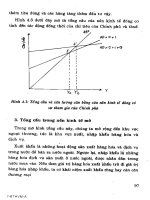
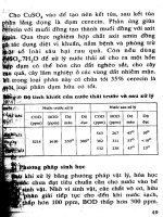


![[Triết Học] Triết Học Lenin - Học Thuyết Marx tập 18 phần 5 pptx](https://media.store123doc.com/images/document/2014_08/01/medium_wum1406881231.jpg)