Foundations of Technical Analysis:
Computational Algorithms, Statistical
Inference, and Empirical Implementation
ANDREW W. LO, HARRY MAMAYSKY, AND JIANG WANG*
ABSTRACT
Technical analysis, also known as “charting,” has been a part of financial practice
for many decades, but this discipline has not received the same level of academic
scrutiny and acceptance as more traditional approaches such as fundamental analy-
sis. One of the main obstacles is the highly subjective nature of technical analy-
sis—the presence of geometric shapes in historical price charts is often in the eyes
of the beholder. In this paper, we propose a systematic and automatic approach to
technical pattern recognition using nonparametric kernel regression, and we apply
this method to a large number of U.S. stocks from 1962 to 1996 to evaluate the
effectiveness of technical analysis. By comparing the unconditional empirical dis-
tribution of daily stock returns to the conditional distribution—conditioned on spe-
cific technical indicators such as head-and-shoulders or double-bottoms—we find
that over the 31-year sample period, several technical indicators do provide incre-
mental information and may have some practical value.
ONE OF THE GREATEST GULFS between academic finance and industry practice
is the separation that exists between technical analysts and their academic
critics. In contrast to fundamental analysis, which was quick to be adopted
by the scholars of modern quantitative finance, technical analysis has been
an orphan from the very start. It has been argued that the difference be-
tween fundamental analysis and technical analysis is not unlike the differ-
ence between astronomy and astrology. Among some circles, technical analysis
is known as “voodoo finance.” And in his inf luential book A Random Walk
down Wall Street, Burton Malkiel ~1996! concludes that “@u#nder scientific
scrutiny, chart-reading must share a pedestal with alchemy.”
However, several academic studies suggest that despite its jargon and meth-
ods, technical analysis may well be an effective means for extracting useful
information from market prices. For example, in rejecting the Random Walk

* MIT Sloan School of Management and Yale School of Management. Corresponding author:
Andrew W. Lo ~!. This research was partially supported by the MIT Laboratory for
Financial Engineering, Merrill Lynch, and the National Science Foundation ~Grant SBR–
9709976!. We thank Ralph Acampora, Franklin Allen, Susan Berger, Mike Epstein, Narasim-
han Jegadeesh, Ed Kao, Doug Sanzone, Jeff Simonoff, Tom Stoker, and seminar participants at
the Federal Reserve Bank of New York, NYU, and conference participants at the Columbia-
JAFEE conference, the 1999 Joint Statistical Meetings, RISK 99, the 1999 Annual Meeting of
the Society for Computational Economics, and the 2000 Annual Meeting of the American Fi-
nance Association for valuable comments and discussion.
THE JOURNAL OF FINANCE • VOL. LV, NO. 4 • AUGUST 2000
1705
Hypothesis for weekly U.S. stock indexes, Lo and MacKinlay ~1988, 1999!
have shown that past prices may be used to forecast future returns to some
degree, a fact that all technical analysts take for granted. Studies by Tabell
and Tabell ~1964!, Treynor and Ferguson ~1985!, Brown and Jennings ~1989!,
Jegadeesh and Titman ~1993!, Blume, Easley, and O’Hara ~1994!, Chan,
Jegadeesh, and Lakonishok ~1996!, Lo and MacKinlay ~1997!, Grundy and
Martin ~1998!, and Rouwenhorst ~1998! have also provided indirect support
for technical analysis, and more direct support has been given by Pruitt and
White ~1988!, Neftci ~1991!, Brock, Lakonishok, and LeBaron ~1992!, Neely,
Weller, and Dittmar ~1997!, Neely and Weller ~1998!, Chang and Osler ~1994!,
Osler and Chang ~1995!, and Allen and Karjalainen ~1999!.
One explanation for this state of controversy and confusion is the unique
and sometimes impenetrable jargon used by technical analysts, some of which
has developed into a standard lexicon that can be translated. But there are
many “homegrown” variations, each with its own patois, which can often
frustrate the uninitiated. Campbell, Lo, and MacKinlay ~1997, 43–44! pro-
vide a striking example of the linguistic barriers between technical analysts
and academic finance by contrasting this statement:
The presence of clearly identified support and resistance levels, coupled

with a one-third retracement parameter when prices lie between them,
suggests the presence of strong buying and selling opportunities in the
near-term.
with this one:
The magnitudes and decay pattern of the first twelve autocorrelations
and the statistical significance of the Box-Pierce Q-statistic suggest the
presence of a high-frequency predictable component in stock returns.
Despite the fact that both statements have the same meaning—that past
prices contain information for predicting future returns—most readers find
one statement plausible and the other puzzling or, worse, offensive.
These linguistic barriers underscore an important difference between tech-
nical analysis and quantitative finance: technical analysis is primarily vi-
sual, whereas quantitative finance is primarily algebraic and numerical.
Therefore, technical analysis employs the tools of geometry and pattern rec-
ognition, and quantitative finance employs the tools of mathematical analy-
sis and probability and statistics. In the wake of recent breakthroughs in
financial engineering, computer technology, and numerical algorithms, it is
no wonder that quantitative finance has overtaken technical analysis in
popularity—the principles of portfolio optimization are far easier to pro-
gram into a computer than the basic tenets of technical analysis. Neverthe-
less, technical analysis has survived through the years, perhaps because its
visual mode of analysis is more conducive to human cognition, and because
pattern recognition is one of the few repetitive activities for which comput-
ers do not have an absolute advantage ~yet!.
1706 The Journal of Finance
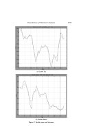
Indeed, it is difficult to dispute the potential value of price0volume charts
when confronted with the visual evidence. For example, compare the two
hypothetical price charts given in Figure 1. Despite the fact that the two
price series are identical over the first half of the sample, the volume pat-
terns differ, and this seems to be informative. In particular, the lower chart,

which shows high volume accompanying a positive price trend, suggests that
there may be more information content in the trend, e.g., broader partici-
pation among investors. The fact that the joint distribution of prices and
volume contains important information is hardly controversial among aca-
demics. Why, then, is the value of a visual depiction of that joint distribution
so hotly contested?
Figure 1. Two hypothetical price/volume charts.
Foundations of Technical Analysis 1707
In this paper, we hope to bridge this gulf between technical analysis and
quantitative finance by developing a systematic and scientific approach to
the practice of technical analysis and by employing the now-standard meth-
ods of empirical analysis to gauge the efficacy of technical indicators over
time and across securities. In doing so, our goal is not only to develop a
lingua franca with which disciples of both disciplines can engage in produc-
tive dialogue but also to extend the reach of technical analysis by augment-
ing its tool kit with some modern techniques in pattern recognition.
The general goal of technical analysis is to identify regularities in the time
series of prices by extracting nonlinear patterns from noisy data. Implicit in
this goal is the recognition that some price movements are significant—they
contribute to the formation of a specific pattern—and others are merely ran-
dom f luctuations to be ignored. In many cases, the human eye can perform this
“signal extraction” quickly and accurately, and until recently, computer algo-
rithms could not. However, a class of statistical estimators, called smoothing
estimators, is ideally suited to this task because they extract nonlinear rela-
tions [m~{! by “averaging out” the noise. Therefore, we propose using these es-
timators to mimic and, in some cases, sharpen the skills of a trained technical
analyst in identifying certain patterns in historical price series.
In Section I, we provide a brief review of smoothing estimators and de-
scribe in detail the specific smoothing estimator we use in our analysis:
kernel regression. Our algorithm for automating technical analysis is de-

scribed in Section II. We apply this algorithm to the daily returns of several
hundred U.S. stocks from 1962 to 1996 and report the results in Section III.
To check the accuracy of our statistical inferences, we perform several Monte
Carlo simulation experiments and the results are given in Section IV. We
conclude in Section V.
I. Smoothing Estimators and Kernel Regression
The starting point for any study of technical analysis is the recognition that
prices evolve in a nonlinear fashion over time and that the nonlinearities con-
tain certain regularities or patterns. To capture such regularities quantita-
tively, we begin by asserting that prices $P
t
% satisfy the following expression:
P
t
ϭ m~X
t
! ϩ e
t
, t ϭ 1, ,T, ~1!
where m~X
t
! is an arbitrary fixed but unknown nonlinear function of a state
variable X
t
and $e
t
% is white noise.
For the purposes of pattern recognition in which our goal is to construct a
smooth function [m~{! to approximate the time series of prices $ p
t

%,weset
the state variable equal to time, X
t
ϭ t. However, to keep our notation con-
sistent with that of the kernel regression literature, we will continue to use
X
t
in our exposition.
When prices are expressed as equation ~1!, it is apparent that geometric
patterns can emerge from a visual inspection of historical price series—
prices are the sum of the nonlinear pattern m~X
t
! and white noise—and
1708 The Journal of Finance
that such patterns may provide useful information about the unknown func-
tion m~{! to be estimated. But just how useful is this information?
To answer this question empirically and systematically, we must first de-
velop a method for automating the identification of technical indicators; that
is, we require a pattern-recognition algorithm. Once such an algorithm is
developed, it can be applied to a large number of securities over many time
periods to determine the efficacy of various technical indicators. Moreover,
quantitative comparisons of the performance of several indicators can be
conducted, and the statistical significance of such performance can be as-
sessed through Monte Carlo simulation and bootstrap techniques.
1
In SectionI.A, weprovide a brief reviewof ageneral class of pattern-recognition
techniques known as smoothing estimators, and in Section I.B we describe in
some detail a particular method called nonparametric kernel regression on which
our algorithm is based. Kernel regression estimators are calibrated by a band-
width parameter, and we discuss how the bandwidth is selected in Section I.C.

A. Smoothing Estimators
One of the most common methods for estimating nonlinear relations such
as equation ~1! is smoothing, in which observational errors are reduced by
averaging the data in sophisticated ways. Kernel regression, orthogonal se-
ries expansion, projection pursuit, nearest-neighbor estimators, average de-
rivative estimators, splines, and neural networks are all examples of smoothing
estimators. In addition to possessing certain statistical optimality proper-
ties, smoothing estimators are motivated by their close correspondence to
the way human cognition extracts regularities from noisy data.
2
Therefore,
they are ideal for our purposes.
To provide some intuition for how averaging can recover nonlinear rela-
tions such as the function m~{! in equation ~1!, suppose we wish to estimate
m~{! at a particular date t
0
when X
t
0
ϭ x
0
. Now suppose that for this one
observation, X
t
0
, we can obtain repeated independent observations of the
price P
t
0
, say P

t
0
1
ϭ p
1
, ,P
t
0
n
ϭ p
n
~note that these are n independent real-
izations of the price at the same date t
0
, clearly an impossibility in practice,
but let us continue this thought experiment for a few more steps!. Then a
natural estimator of the function m~{! at the point x
0
is
[m~x
0
! ϭ
1
n
(
iϭ1
n
p
i
ϭ

1
n
(
iϭ1
n
@m~x
0
! ϩ e
t
i
#~2!
ϭm~x
0
!ϩ
1
n
(
iϭ1
n
e
t
i
, ~3!
1
A similar approach has been proposed by Chang and Osler ~1994! and Osler and Chang
~1995! for the case of foreign-currency trading rules based on a head-and-shoulders pattern.
They develop an algorithm for automatically detecting geometric patterns in price or exchange
data by looking at properly defined local extrema.
2
See, for example, Beymer and Poggio ~1996!, Poggio and Beymer ~1996!, and Riesenhuber

and Poggio ~1997!.
Foundations of Technical Analysis 1709
and by the Law of Large Numbers, the second term in equation ~3! becomes
negligible for large n.
Of course, if $P
t
% is a time series, we do not have the luxury of repeated
observations for a given X
t
. However, if we assume that the function m~{! is
sufficiently smooth, then for time-series observations X
t
near the value x
0
,
the corresponding values of P
t
should be close to m~x
0
!. In other words, if
m~{! is sufficiently smooth, then in a small neighborhood around x
0
, m~x
0
!
will be nearly constant and may be estimated by taking an average of the P
t
s
that correspond to those X
t

s near x
0
. The closer the X
t
s are to the value x
0
,
the closer an average of corresponding P
t
s will be to m~x
0
!. This argues for
a weighted average of the P
t
s, where the weights decline as the X
t
s get
farther away from x
0
. This weighted-average or “local averaging” procedure
of estimating m~x! is the essence of smoothing.
More formally, for any arbitrary x, a smoothing estimator of m~x! may be
expressed as
[m~x![
1
T
(
tϭ1
T
v

t
~x!P
t
, ~4!
where the weights $v
t
~x!% are large for those P
t
s paired with X
t
s near x, and
small for those P
t
s with X
t
s far from x. To implement such a procedure, we
must define what we mean by “near” and “far.” If we choose too large a
neighborhood around x to compute the average, the weighted average will be
too smooth and will not exhibit the genuine nonlinearities of m~{!.Ifwe
choose too small a neighborhood around x, the weighted average will be too
variable, ref lecting noise as well as the variations in m~{!. Therefore, the
weights $v
t
~x!% must be chosen carefully to balance these two considerations.
B. Kernel Regression
For the kernel regression estimator, the weight function v
t
~x! is con-
structed from a probability density function K~x!, also called a kernel:
3

K~x! Ն 0,
͵
K~u! du ϭ 1. ~5!
By rescaling the kernel with respect to a parameter h Ͼ 0, we can change its
spread; that is, let
K
h
~u![
1
h
K~u0h!,
͵
K
h
~u!du ϭ 1 ~6!
3
Despite the fact that K~x! is a probability density function, it plays no probabilistic role in
the subsequent analysis—it is merely a convenient method for computing a weighted average
and does not imply, for example, that X is distributed according to K~x!~which would be a
parametric assumption!.
1710 The Journal of Finance
and define the weight function to be used in the weighted average ~equation
~4!! as
v
t, h
~x![K
h
~xϪX
t
!0g

h
~x!, ~7!
g
h
~x![
1
T
(
tϭ1
T
K
h
~xϪX
t
!. ~8!
If h is very small, the averaging will be done with respect to a rather small
neighborhood around each of the X
t
s. If h is very large, the averaging will be
over larger neighborhoods of the X
t
s. Therefore, controlling the degree of
averaging amounts to adjusting the smoothing parameter h, also known as
the bandwidth. Choosing the appropriate bandwidth is an important aspect
of any local-averaging technique and is discussed more fully in Section II.C.
Substituting equation ~8! into equation ~4! yields the Nadaraya–Watson
kernel estimator [m
h
~x! of m~x!:
[m

h
~x! ϭ
1
T
(
tϭ1
T
v
t, h
~x!Y
t
ϭ
(
tϭ1
T
K
h
~x Ϫ X
t
!Y
t
(
tϭ1
T
K
h
~x Ϫ X
t
!
. ~9!

Under certain regularity conditions on the shape of the kernel K and the
magnitudes and behavior of the weights as the sample size grows, it may be
shown that [m
h
~x! converges to m~x! asymptotically in several ways ~see
Härdle ~1990! for further details!. This convergence property holds for a
wide class of kernels, but for the remainder of this paper we shall use the
most popular choice of kernel, the Gaussian kernel:
K
h
~x! ϭ
1
h% 2p
e
Ϫx
2
0 2h
2
~10!
C. Selecting the Bandwidth
Selecting the appropriate bandwidth h in equation ~9! is clearly central to
the success of [m
h
~{! in approximating m~{!—too little averaging yields a
function that is too choppy, and too much averaging yields a function that is
too smooth. To illustrate these two extremes, Figure 2 displays the Nadaraya–
Watson kernel estimator applied to 500 data points generated from the relation:
Y
t
ϭ Sin~X

t
! ϩ 0.5eZ
t
, eZ
t
; N ~0,1!, ~11!
where X
t
is evenly spaced in the interval @0,2p#. Panel 2 ~a! plots the raw
data and the function to be approximated.
Foundations of Technical Analysis 1711
(a)
(b)
Figure 2. Illustration of bandwidth selection for kernel regression.
1712 The Journal of Finance
(c)
(d)
Figure 2. Continued
Foundations of Technical Analysis 1713
Kernel estimators for three different bandwidths are plotted as solid lines in
Panels 2~b!–~c!. The bandwidth in 2~b! is clearly too small; the function is too
variable, fitting the “noise” 0.5eZ
t
and also the “signal” Sin~{!. Increasing the
bandwidth slightly yields a much more accurate approximation to Sin ~{! as
Panel 2~c! illustrates. However, Panel 2~d! shows that if the bandwidth is in-
creased beyond some point, there is too much averaging and information is lost.
There are several methods for automating the choice of bandwidth h in
equation ~9!, but the most popular is the cross-validation method in which h
is chosen to minimize the cross-validation function

CV~h! ϭ
1
T
(
tϭ1
T
~P
t
Ϫ [m
h, t
!
2
, ~12!
where
[m
h, t
[
1
T
(
tt
T
v
t, h
Y
t
. ~13!
The estimator [m
h, t
is the kernel regression estimator applied to the price

history $P
t
% with the tth observation omitted, and the summands in equa-
tion ~12! are the squared errors of the [m
h, t
s, each evaluated at the omitted
observation. For a given bandwidth parameter h, the cross-validation func-
tion is a measure of the ability of the kernel regression estimator to fit each
observation P
t
when that observation is not used to construct the kernel
estimator. By selecting the bandwidth that minimizes this function, we ob-
tain a kernel estimator that satisfies certain optimality properties, for ex-
ample, minimum asymptotic mean-squared error.
4
Interestingly, the bandwidths obtained from minimizing the cross-validation
function are generally too large for our application to technical analysis—
when we presented several professional technical analysts with plots of cross-
validation-fitted functions [m
h
~{!, they all concluded that the fitted functions
were too smooth. In other words, the cross-validation-determined bandwidth
places too much weight on prices far away from any given time t, inducing
too much averaging and discarding valuable information in local price move-
ments. Through trial and error, and by polling professional technical ana-
lysts, we have found that an acceptable solution to this problem is to use a
bandwidth of 0.3 ϫ h
*
, where h
*

minimizes CV~h!.
5
Admittedly, this is an ad
hoc approach, and it remains an important challenge for future research to
develop a more rigorous procedure.
4
However, there are other bandwidth-selection methods that yield the same asymptotic op-
timality properties but that have different implications for the finite-sample properties of ker-
nel estimators. See Härdle ~1990! for further discussion.
5
Specifically, we produced fitted curves for various bandwidths and compared their extrema
to the original price series visually to see if we were fitting more “noise” than “signal,” and we
asked several professional technical analysts to do the same. Through this informal process, we
settled on the bandwidth of 0.3 ϫ h
*
and used it for the remainder of our analysis. This pro-
cedure was followed before we performed the statistical analysis of Section III, and we made no
revision to the choice of bandwidth afterward.
1714 The Journal of Finance