Engineering Analysis with Ansys Software Episode 1 Part 6 ppsx
Bạn đang xem bản rút gọn của tài liệu. Xem và tải ngay bản đầy đủ của tài liệu tại đây (1.16 MB, 20 trang )
Ch03-H6875.tex 24/11/2006 17: 2 page 84
84 Chapter 3 Application of ANSYS to stress analysis
circular areas from the larger rectangular area to create a stepped beam area with
a rounded fillet as shown in Figure 3.54.
Figure 3.54 A stepped cantilever beam area with a rounded fillet.
A3.2.1 HOW TO DISPLAY AREA NUMBERS
Area numbers can be displayed in the “ANSYS Graphics” window by the following
procedure.
Command
ANSYS Utility Menu →PlotCtrls →Numbering
(1) The Plot Numbering Controls window opens as shown in Figure 3.29.
(2) Click AREA
Off box to change it to
✓ On box.
(3) Click OK button to display area numbers in the corresponding areas in theANSYS
Graphics window.
(4) To delete the area numbers, click AREA
✓ On box again to change it to
Off
box.
3.2 The principle of St. Venant
3.2.1 Example problem
An elastic strip subjected to distributed uniaxial tensile stress or negative pressure at
one end and clamped at the other end.
Ch03-H6875.tex 24/11/2006 17: 2 page 85
3.2 The principle of St. Venant 85
Perform an FEM analysis of a 2-D elastic strip subjected to a distributed stress
in the longitudinal direction at one end and clamped at the other end (shown in
Figure 3.55 below) and calculate the stress distributions along the cross sections at
different distances from the loaded end in the strip.
Triangular distribution of stress σ
0
200 mm
20 mm
10 MPa
Figure 3.55 A 2-D elastic strip subjected to a distributed force in the longitudinal direction at one end and
clamped at the other end.
3.2.2 Problem description
Geometry: length l =200 mm, height h =20 mm, thickness b =10 mm.
Material: mild steel having Young’s modulus E =210 GPa and Poisson’s ratio ν =0.3.
Boundary conditions: The elastic strip is subjected to a triangular distribution of
stress in the longitudinal direction at the right end and clamped to a rigid wall at the
left end.
3.2.3
Analytical procedures
3.2.3.1 C
REATION OF AN ANALYTICAL MODEL
Command
ANSYS Main Menu →Preprocessor →Modeling →Create →Areas →
Rectangle →By2Corners
(1) Input two 0’s into the “WP X” and “WP Y” boxes in the “Rectangle by 2 Cor-
ners” window to determine the lower left corner point of the elastic strip on the
Cartesian coordinates of the working plane.
(2) Input 200 and 20 (mm) into the Width and Height boxes, respectively, to
determine the shape of the elastic strip model.
(3) Click the OK button to create the rectangular area, or beam on the ANSYS
Graphics window.
Ch03-H6875.tex 24/11/2006 17: 2 page 86
86 Chapter 3 Application of ANSYS to stress analysis
In the procedures above, the geometry of the strip is input in millimeters. You
must decide what kind of units to use in finite-element analyses. When you input
the geometry of a model to analyze in millimeters, for example, you must input
applied loads in N (Newton) and Young’s modulus in MPa, since 1 MPa is equivalent
to 1 N/mm
2
. When you use meters and N as the units of length and load, respectively,
you must input Young’s modulus in Pa, since 1 Pa is equivalent to 1 N/m
2
. You can
choose any system of unit you would like to, but your unit system must be consistent
throughout the analyses.
3.2.3.2 INPUT OF THE ELASTIC PROPERTIES OF THE STRIP MATERIAL
Command
ANSYS Main Menu →Preprocessor →Material Props →Material Models
(1) The Define Material Model Behavior window opens.
(2) Double-click Structural, Linear, Elastic, and Isotropic buttons one after another.
(3) Input the value of Young’s modulus, 2.1e5 (MPa), and that of Poisson’s ratio,
0.3, into EX and PRXY boxes, and click the OK button of the Linear Isotropic
Properties for Materials Number 1 window.
(4) Exit from the Define Material Model Behavior window by selecting Exit in the
Material menu of the window.
3.2.3.3 FINITE-ELEMENT DISCRETIZATION OF THE STRIP AREA
[1] Selection of the element type
Command
ANSYS Main Menu →Preprocessor →Element Type →Add/Edit/Delete
(1) The Element Types window opens.
(2) Click the Add … button in the Element Types window to open the Library of
Element Types window and select the element type to use.
(3) Select Structural Mass – Solid and Quad 8node 82.
(4) Click the OK button in the Library of Element Types window to use the 8-node
isoparametric element.
(5) Click the Options … button in the Element Types window to open the PLANE82
element type options window. Select the Plane strs w/thk item in the Element
behavior box and click the OK buttontoreturntotheElement Types window.
Click the Close button in the Element Types window to close the window.
[2] Input of the element thickness
Command
ANSYS Main Menu →Preprocessor →Real Constants →Add/Edit/Delete
(1) The Real Constants window opens.
(2) Click [A] Add/Edit/Delete buttontoopentheReal Constants window and click
the Add … button.
Ch03-H6875.tex 24/11/2006 17: 2 page 87
3.2 The principle of St. Venant 87
(3) The Element Type for Real Constants window opens. Click the OK button.
(4) The Element Type for Real Constants window vanishes and the Real Constants
Set Number 1. for PLANE82 window appears instead. Input a strip thickness of
10 (mm) in the Thickness box and click the OK button.
(5) The Real Constants window returns with the display of the Defined Real
Constants Sets box changed to Set 1. Click the Close button.
[3] Sizing of the elements
Command
ANSYS Main Menu →Preprocessor →Meshing →Size Cntrls →Manual Size →
Global →Size
(1) The Global Element Sizes window opens.
(2) Input 2 in the SIZE box and click the OK button.
[4] Dividing the right-end side of the strip area into two lines
Before proceeding to meshing, the right-end side of the strip area must be divided
into two lines for imposing the triangular distribution of the applied stress or pressure
by executing the following commands.
Command
Figure 3.56 “Divide Mul-
tiple Lines ” window.
ANSYS Main Menu →Preprocessor →
Modeling →Operate →Booleans →Divide →
Lines w/Options
(1) The Divide Multiple Lines … window opens as
shown in Figure 3.56.
(2) When the mouse cursor is moved to the ANSYS
Graphics window,an upward arrow (↑) appears.
(3) Confirming that the Pick and Single buttons are
selected, move the upward arrow onto the right-
end side of the strip area and click the left button
of the mouse.
(4) Click the OK button in the Divide Multiple
Lines window to display the Divide Multiple
Lines with Options window as shown in Figure
3.57.
(5) Input 2 in [A] NDIV box and 0.5 in [B] RATIO
box, and select Be modified in [C] KEEP box.
(6) Click [D] OK button.
[5] Meshing
Command
ANSYS Main Menu →Preprocessor →Meshing →
Mesh →Areas →Free
(1) The Mesh Areas window opens.
Ch03-H6875.tex 24/11/2006 17: 2 page 88
88 Chapter 3 Application of ANSYS to stress analysis
A
B
C
D
Figure 3.57 “Divide Multiple Lines with Options” window.
(2) The upward arrow appears in the ANSYS Graphics window. Move this arrow to
the elastic strip area and click this area.
(3) The color of the area turns from light blue into pink. Click the OK buttontosee
the area meshed by 8-node rectangular isoparametric finite elements.
3.2.3.4 INPUT OF BOUNDARY CONDITIONS
[1] Imposing constraint conditions on the left end of the strip
Command
ANSYS Main Menu →Solution →Define Loads →Apply →Structural →
Displacement →On Lines
(1) The Apply U. ROT on Lines window opens and the upward arrow appears when
the mouse cursor is moved to the ANSYS Graphics window.
(2) Confirming that the Pick and Single buttons are selected, move the upward arrow
onto the left-end side of the strip area and click the left button of the mouse.
(3) Click the OK button in the Apply U. ROT on Lines window to display another
Apply U. ROT on Lines window.
(4) Select ALL DOF in the Lab2 box and click OK button in the Apply U. ROT on
Lines window.
[2] Imposing a triangular distribution of applied stress on the right end of the strip
Distributed load or stress can be defined by pressure on lines and the triangular
distribution of appliedloadcanbedefined as thecompositeof two lineardistributions
Ch03-H6875.tex 24/11/2006 17: 2 page 89
3.2 The principle of St. Venant 89
of pressure which are symmetric to each other with respect to the center line of the
strip area.
Command
ANSYS Main Menu →Solution →Define Loads →Apply →Structural →
Pressure →On Lines
Figure 3.58 “Apply PRES on Lines”
window for picking the lines
to which pressure is applied.
(1) The Apply PRES on Lines window opens (see
Figure 3.58) and the upward arrow appears
when the mouse cursor is moved to the ANSYS
Graphics window.
(2) Confirming that the Pick and Single buttons are
selected, move the upward arrow onto the upper
line of the right-end side of the strip area and
click the left button of the mouse. Then, click the
OK button. Remember that the right-end side
of the strip area was divided into two lines in
Procedure [4] in the preceding Section 3.2.3.3.
(3) Another Apply PRES on Lines window opens
(see Figure 3.59). Select Constant value in [A]
[SFL] Apply PRES on lines as a box and input
[B] −10 (MPa) in VALUE Load PRES value box
and [C] 0 (MPa) in Va l u e box.
(4) Click [D] OK button in the window to define
a linear distribution of pressure on the upper
line which is zero at the upper right corner and
−10 (MPa) at the center of the right-end side of
the strip area (see Figure 3.60).
(5) For thelower lineof theright-end sideof thestrip
area,repeat thecommands aboveandProcedures
(2) through (4).
(6) Select Constant value in [A] [SFL] Apply PRES on lines as a box and input [B]
0 (MPa) in VALUE Load PRES value box and [C] −10 (MPa) in Va l ue box as
shown in Figure 3.61. Note that the values to input in the lower two boxes in the
Apply PRES on Lines window is interchanged, since the distributed pressure on
the lower line of the right-end side of the strip area is symmetric to that on the
upper line with respect to the center line of the strip area.
(7) Click [D] OK button in the window shown in Figure 3.60 to define a linear
distribution of pressure on the lower line which is −10 MPa at the center and
zero at the lower right corner of the right-end side of the strip area as shown in
Figure 3.62.
3.2.3.5 SOLUTION PROCEDURES
Command
ANSYS Main Menu →Solution →Solve →Current LS
Ch03-H6875.tex 24/11/2006 17: 2 page 90
90 Chapter 3 Application of ANSYS to stress analysis
A
B
C
D
Figure 3.59 “Apply PRES on Lines” window for applying linearly distributed pressure to the upper half of
the right end of the elastic strip.
Figure 3.60 Linearly distributed negative pressure applied to the upper half of the right-end side of the
elastic strip.
Ch03-H6875.tex 24/11/2006 17: 2 page 91
3.2 The principle of St. Venant 91
A
B
C
D
Figure 3.61 “Apply PRES on Lines” window for applying linearly distributed pressure to the lower half of
the right end of the elastic strip.
Figure 3.62 Triangular distribution of pressure applied to the right end of the elastic strip.
(1) The Solve Current Load Step and /STATUS Command windows appear.
(2) Click the OK button in the Solve Current Load Step window to begin the solution
of the current load step.
Ch03-H6875.tex 24/11/2006 17: 2 page 92
92 Chapter 3 Application of ANSYS to stress analysis
(3) Select the File button in /STATUS Command window to open the submenu and
select the Close button to close the /STATUS Command window.
(4) When solution is completed, the Note window appears. Click the Close button
to close the “Note” window.
3.2.3.6 CONTOUR PLOT OF STRESS
Command
ANSYS Main Menu →General Postproc →Plot Results →Contour Plot →Nodal
Solution
(1) The Contour Nodal Solution Data window opens.
(2) Select Stress and X-Component of stress.
(3) Click the OK button to display the contour of the x-component of stress in the
elastic strip in the ANSYS Graphics window as shown in Figure 3.63.
Figure 3.63 Contour of the x-component of stress in the elastic strip showing uniform stress distribution
at one width or larger distance from the right end of the elastic strip to which triangular
distribution of pressure is applied.
3.2.4 Discussion
Figure 3.64 shows the variations of the longitudinal stress distribution in the cross
section with the x-position of the elastic strip. At the right end of the strip, or at
Ch03-H6875.tex 24/11/2006 17: 2 page 93
3.3 Stress concentration due to elliptic holes 93
0 5 10
0
5
10
15
20
x (mm)
200
190
180
100
Longitudinal stress, σ
x
(MPa)
y-coordinate, y (mm)
Figure 3.64 Variations of the longitudinal stress distribution in the cross section with the x-position of the
elastic strip.
x =200 mm, the distribution of the applied longitudinal stress takes the triangular
shape which is zero at the upper and lower corners and 10 MPa at the center of the
strip. The longitudinal stress distribution varies as the distance of the cross section
from the right end of the strip increases, and the distribution becomes almost uniform
at x =180 mm, i.e., at one width distance from the end of the stress application. The
total amount of stress in any cross section is the same, i.e., 1 kN in the strip and, stress
is uniformly distributed and the magnitude of stress becomes 5MPa at any cross
section at one width or larger distance from the end of the stress application.
The above result is known as the principle of St. Venant and is very useful in
practice, or in the design of structural components. Namely, even if the stress dis-
tribution is very complicated at the loading points due to the complicated shape of
load transfer equipment, one can assume a uniform stress distribution in the main
parts of structural components or machine elements at some distance from the load
transfer equipment.
3.3
Stress concentration due to elliptic holes
3.3.1 Example problem
An elastic plate with an elliptic hole in its center is subjected to uniform longitudinal
tensile stress σ
0
at one end and clamped at the other end in Figure 3.65. Perform the
FEM stress analysis of the 2-D elastic plate and calculate the maximum longitudinal
stress σ
max
in the plate to obtain the stress concentration factor α =σ
max
/σ
0
. Observe
the variation of the longitudinal stress distribution in the ligament between the foot
of the hole and the edge of the plate.
Ch03-H6875.tex 24/11/2006 17: 2 page 94
94 Chapter 3 Application of ANSYS to stress analysis
Uniform longitudinal stress σ
0
400 mm
200 mm 200 mm
B
A
100 mm
10 mm
20 mm
Figure 3.65 A 2-D elastic plate with an elliptic hole in its center subjected to a uniform longitudinal stress
at one end and clamped at the other end.
3.3.2 Problem description
Plate geometry: l =400 mm, height h =100 mm, thickness b =10 mm.
Material: mild steel having Young’s modulus E =210 GPa and Poisson’s ratio ν =0.3.
Elliptic hole: An elliptic hole has a minor radius of 5 mm in the longitudinal direction
and a major radius of 10 mm in the transversal direction.
Boundary conditions: The elastic plate is subjected to a uniform tensile stress of
σ
0
=10 Mpa in the longitudinal direction at the right end and clamped to a rigid wall
at the left end.
3.3.3 Analytical procedures
3.3.3.1 CREATION OF AN ANALYTICAL MODEL
Let us use a quarter model of the elastic plate with an elliptic hole as illustrated later in
Figure 3.70, since the plate is symmetric about the horizontal and vertical centerlines.
The quarter model can be created by a slender rectangular area from which an elliptic
area is subtracted by using the Boolean operation described in Section A3.1.
First, create the rectangular area by the following operation:
Command
ANSYSMain Menu →Preprocessor →Modeling →Create →Areas →Rectangle →
By2Corners
(1) Input two 0’s into the WP X and WP Y boxes in the Rectangle by 2 Corners win-
dow to determine the lower left corner point of the elastic plate on the Cartesian
coordinates of the working plane.
Ch03-H6875.tex 24/11/2006 17: 2 page 95
3.3 Stress concentration due to elliptic holes 95
(2) Input 200 and 50 (mm) into the Width and Height boxes, respectively, to
determine the shape of the quarter elastic plate model.
(3) Click the OK button to create the quarter elastic plate on the ANSYS Graphics
window.
Then, create a circular area having a diameter of 10 mm and then reduce its
diameter in the longitudinal direction to a half of the original value to get the elliptic
area. The following commands create a circular area by designating the coordinates
(UX, UY) of the center and the radius of the circular area:
Command
A
B
C
D
Figure 3.66 “Solid Circular Area”
window.
ANSYS Main Menu →Preprocessor →Modeling →Create →Areas →Circle →
Solid Circle
(1) The Solid Circular Area window
opens as shown in Figure 3.66.
(2) Input two 0’s into [A] WP X and [B]
WP Y boxes to determine the center
position of the circular area.
(3) Input [C] 10 (mm) in Radius box to
determine the radius of the circular
area.
(4) Click [D] OK buttontocreate
the circular area superimposed on
the rectangular area in the ANSYS
Graphics window as shown in Fig-
ure 3.67.
In order to reduce the diameter of the
circular area in the longitudinal direction
to a half of the original value, use the
following Scale →Areas operation:
Command
ANSYS Main Menu →Preprocessor →
Modeling →Operate →Scale →Areas
(1) The Scale Areas window opens as shown in Figure 3.68.
(2) The upward arrow appears in the ANSYS Graphics window. Move the arrow to
the circular area and pick it by clicking the left button of the mouse. The color
of the circular area turns from light blue into pink and click [A] OK button.
(3) The color of the circular area turns into light blue and another Scale Areas
window opens as shown in Figure 3.69.
(4) Input [A] 0.5 in RX box, select [B] Areas only in NOELEM box and [C] Moved
in IMOVE box.
(5) Click [D] OK button. An elliptic area appears and the circular area still remains.
The circular area is an afterimage and does not exist in reality. To erase this
Ch03-H6875.tex 24/11/2006 17: 2 page 96
96 Chapter 3 Application of ANSYS to stress analysis
Figure 3.67 Circular area superimposed on the rectangular area.
A
Figure 3.68 “Scale Areas”
window.
A
B
C
D
Figure 3.69 “Scale Areas”.
Ch03-H6875.tex 24/11/2006 17: 2 page 97
3.3 Stress concentration due to elliptic holes 97
after-image, perform the following commands:
Command
ANSYS Utility Menu →Plot →Replot
The circular area vanishes. Subtract the elliptic area from the rectangular area in a
similar manner as described in Section A3.2, i.e.,
Command
ANSYS Main Menu →Preprocessor →Modeling →Operate →Booleans →
Subtract →Areas
(1) Pick the rectangular area by the upward arrow and confirm that the color of the
area picked turns from light blue into pink. Click the OK button.
(2) Pick the elliptic area by the upward arrow and confirm that the color of the elliptic
area picked turns from light blue into pink. Click the OK buttontosubtractthe
elliptic area from the rectangular area to get a quarter model of a plate with an
elliptic hole in its center as shown in Figure 3.70.
Figure 3.70 Quarter model of a plate with an elliptic hole in its center created by subtracting an elliptic
area from a rectangular area.
3.3.3.2 I
NPUT OF THE ELASTIC PROPERTIES OF THE PLATE MATERIAL
Command
ANSYS Main Menu →Preprocessor →Material Props →Material Models
(1) The Define Material Model Behavior window opens.
(2) Double-click Structural, Linear, Elastic, and Isotropic buttons one after another.
Ch03-H6875.tex 24/11/2006 17: 2 page 98
98 Chapter 3 Application of ANSYS to stress analysis
(3) Input the value of Young’s modulus, 2.1e5 (MPa), and that of Poisson’s ratio,
0.3, into EX and PRXY boxes, and click the OK button of the Linear Isotropic
Properties for Materials Number 1 window.
(4) Exit from the Define Material Model Behavior window by selecting Exit in the
Material menu of the window.
3.3.3.3 FINITE-ELEMENT DISCRETIZATION OF THE QUARTER PLATE AREA
[1] Selection of the element type
Command
ANSYS Main Menu →Preprocessor →Element Type →Add/Edit/Delete
(1) The Element Types window opens.
(2) Click the Add button in the Element Types window to open the Library of
Element Types window and select the element type to use.
(3) Select Structural Mass – Solid and Quad 8node 82.
(4) Click the OK button in the Library of Element Types window to use the 8-node
isoparametric element.
(5) Click the Options … button in the Element Types window to open the PLANE82
element type options window. Select the Plane strs w/thk item in the Element
behavior box and click the OK buttontoreturntotheElement Types window.
Click the Close button in the Element Types window to close the window.
[2] Input of the element thickness
Command
ANSYS Main Menu →Preprocessor →Real Constants →Add/Edit/Delete
(1) The Real Constants window opens.
(2) Click [A] Add/Edit/Delete buttontoopentheReal Constants window and
click the Add button.
(3) The Element Type for Real Constants window opens. Click the OK button.
(4) The Element Type for Real Constants window vanishes and the Real Constants
Set Number 1. for PLANE82 window appears instead. Input a strip thickness of
10 (mm) in the Thickness box and click the OK button.
(5) The Real Constants window returns with the display of the Defined Real
Constants Sets box changed to Set 1. Click the Close button.
[3] Sizing of the elements
Command
ANSYS Main Menu →Preprocessor →Meshing →Size Cntrls →Manual Size →
Global →Size
(1) The Global Element Sizes window opens.
(2) Input 1.5 in the SIZE box and click the OK button.
Ch03-H6875.tex 24/11/2006 17: 2 page 99
3.3 Stress concentration due to elliptic holes 99
[4] Meshing
Command
ANSYS Main Menu →Preprocessor →Meshing →Mesh →Areas →Free
(1) The Mesh Areas window opens.
(2) The upward arrow appears in the ANSYS Graphics window. Move this arrow
to the quarter plate area and click this area.
(3) The color of the area turns from light blue into pink. Click the OK buttontosee
the area meshed by 8-node isoparametric finite elements as shown in Figure 3.71.
Figure 3.71 Quarter model of a plate with an elliptic hole meshed by 8-node isoparametric finite elements.
3.3.3.4 INPUT OF BOUNDARY CONDITIONS
[1] Imposing constraint conditions on the left end and the bottom side of the
quarter plate model
Due to the symmetry, the constraint conditions of the quarter plate model are
UX-fixed condition on the left end and UY-fixed condition on the bottom side of the
quarter plate model. Apply the constraint conditions onto the corresponding lines by
the following commands:
Command
ANSYS Main Menu →Solution →Define Loads →Apply →Structural →
Displacement →On Lines
(1) The Apply U. ROT on Lines window opens and the upward arrow appears when
the mouse cursor is moved to the ANSYS Graphics window.
Ch03-H6875.tex 24/11/2006 17: 2 page 100
100 Chapter 3 Application of ANSYS to stress analysis
(2) Confirming that the Pick and Single buttons are selected, move the upward
arrow onto the left-end side of the quarter plate area and click the left button of
the mouse.
(3) Click the OK button in the Apply U. ROT on Lines window to display another
Apply U. ROT on Lines window.
(4) Select UX in the Lab2 box and click the OK button in the Apply U. ROT on Lines
window.
Repeat the commands and operations (1) through (3) above for the bottom side
of the model. Then, select UY in the Lab2 box and click the OK button in the Apply
U. ROT on Lines window.
[2] Imposing a uniform longitudinal stress on the right end of the
quarter plate model
A uniform longitudinal stress can be defined by pressure on the right-end side of the
plate model as described below:
Command
ANSYS Main Menu →Solution →Define Loads →Apply →Structural →
Pressure →On Lines
(1) The Apply PRES on Lines window opens and the upward arrow appears when
the mouse cursor is moved to the ANSYS Graphics window.
(2) Confirming that the Pick and Single buttons are selected, move the upward arrow
onto the right-end side of the quarter plate area and click the left button of the
mouse.
(3) Another Apply PRES on Lines window opens. Select Constant value in the [SFL]
Apply PRES on lines as a box and input −10 (MPa) in the VALUE Load PRES
value box and leave a blank in the Value box.
(4) Click the OK button in the window to define a uniform tensile stress of 10 MPa
applied to the right end of the quarter plate model.
Figure 3.72 illustrates the boundary conditions applied to the center notched plate
model by the above operations.
3.3.3.5 SOLUTION PROCEDURES
Command
ANSYS Main Menu →Solution →Solve →Current LS
(1) The Solve Current Load Step and /STATUS Command windows appear.
(2) Click the OK button in the Solve Current Load Step window to begin the solution
of the current load step.
(3) Select the File button in /STATUS Command window to open the submenu and
select the Close button to close the /STATUS Command window.
(4) When the solution is completed, the Note window appears. Click the Close button
to close the Note window.
Ch03-H6875.tex 24/11/2006 17: 2 page 101
3.3 Stress concentration due to elliptic holes 101
Figure 3.72 Boundary conditions applied to the quarter model of the center notched plate.
3.3.3.6 CONTOUR PLOT OF STRESS
Command
ANSYS Main Menu →General Postproc →Plot Results →Contour Plot →Nodal
Solution
(1) The Contour Nodal Solution Data window opens.
(2) Select Stress and X-Component of stress.
(3) Select Deformed shape with undeformed edge in the Undisplaced shape key
box to compare the shapes of the notched plate before and after deformation.
(4) Click the OK button to display the contour of the x-component of stress in the
quarter model of the center notched plate in the ANSYS Graphics window as
shown in Figure 3.73.
3.3.3.7 OBSERVATION OF THE VARIATION OF THE LONGITUDINAL STRESS
DISTRIBUTION IN THE LIGAMENT REGION
In order to observe the variation of the longitudinal stress distribution in the liga-
ment between the foot of the hole and the edge of the plate, carry out the following
commands:
Command
ANSYS Utility Menu →PlotCtrls →Symbols …
Ch03-H6875.tex 24/11/2006 17: 2 page 102
102 Chapter 3 Application of ANSYS to stress analysis
Figure 3.73 Contour of the x-component of stress in the quarter model of the center notched plate.
The Symbols window opens as shown in Figure 3.74:
(1) Select [A] All Reactions in the [/PBC] Boundary condition symbol buttons,
[B] Pressures in the [/PSF] Surface Load Symbols box and [C] Arrows in the
[/PSF] Show pres and convect as box.
(2) The distributions of the reaction force and the longitudinal stress in the ligament
region (see [A] in Figure 3.75) as well as that of the applied stress on the right
end of the plate area are superimposed on the contour x-component of stress in
the plate in the ANSYS Graphics window. The reaction force is indicated by the
leftward red arrows, whereas the longitudinal stress by the rightward red arrows
in the ligament region.
The longitudinal stress reaches its maximum value at the foot of the hole and is
decreased approaching to a constant value almost equal to the applied stress σ
0
at
some distance, say, about one major diameter distance, from the foot of the hole. This
tendency can be explained by the principle of St. Venant as discussed in the previous
section.
3.3.4 Discussion
If an elliptical hole is placed in an infinite body and subjected to a remote uniform
stress of σ
0
, the maximum stress σ
max
occurs at the foot of the hole, i.e., Point B in
Ch03-H6875.tex 24/11/2006 17: 2 page 103
3.3 Stress concentration due to elliptic holes 103
A
B
C
D
Figure 3.74 “Symbols” window.
Figure 3.65, and is expressed by the following formula:
σ
max
=
1 +2
a
b
σ
0
=
1 +
a
ρ
σ
0
= α
0
σ
0
(3.4)
where a is the major radius, b the minor radius, ρ the local radius of curva-
ture at the foot of the elliptic hole and α
0
the stress concentration factor which is