Ch03-H6875.tex 24/11/2006 17: 2 page 64
64 Chapter 3 Application of ANSYS to stress analysis
(1) Click the upper left point.
(2) Click the lower right point.
Figure 3.24 Magnification of an observation area.
A
B
E
C
D
Figure 3.25 “Apply U. ROT on Nodes” window.
Ch03-H6875.tex 24/11/2006 17: 2 page 65
3.1 Cantilever beam 65
Selection box
Figure 3.26 Picking multiple nodes by box.
nodes can be reset either by picking selected nodes after choosing [E] Unpick button
or clicking the right button of the mouse to turn the upward arrow upside down.
Imposing constraint conditions on nodes
The Apply U. ROT on Nodes window (see Figure 3.27) opens after clicking [C] OK
button in the procedure (2) in the subsection “Selection of nodes” above.
A
B
Figure 3.27 “Apply U. ROT on Nodes” window.
Ch03-H6875.tex 24/11/2006 17: 2 page 66
66 Chapter 3 Application of ANSYS to stress analysis
(1) In case of selecting [A] ALL DOF, the nodes are to be clamped, i.e., the displace-
ments are set to zero in the directions of the x- and y-axes. Similarly, the selection
of UX makes the displacement in the x-direction equal to zero and the selection
of UY makes the displacement in the y-direction equal to zero.
(2) Click [B] OK button and blue triangular symbols, which denote the clamping
conditions, appear in the ANSYS Graphics window as shown in Figure 3.28.

The upright triangles indicate that each node to which the triangular symbol is
attached is fixed in the y-direction, whereas the tilted triangles indicate the fixed
condition in the x-direction.
Figure 3.28 Imposing the clamping conditions on nodes.
How to clear constraint conditions
Command
ANSYS Main Menu →Solution →Define Loads →Delete →Structural →
Displacement →On Nodes
The Delete Node Constrai… window opens.
(1) Click Pick All button to delete the constraint conditions of all the nodes that
the constraint conditions are imposed. Select Single button and pick a particular
node by the upward arrow in the ANSYS Graphics window and click OK button.
(2) The Delete Node constraints window appears. Select ALL DOF and click OK
button to delete the constraint conditions both in the x- and y-directions. Select
UX and UY to delete the constraints in the x- and the y-directions, respectively.
[4] Imposing boundary conditions on nodes
Before imposing load conditions, click Fit button in the Pan-Zoom-Rotate window
(see Figure 3.23) to get the whole view of the area and then zoom in the right end of
the beam area for ease of the following operations.
Ch03-H6875.tex 24/11/2006 17: 2 page 67
3.1 Cantilever beam 67
Selection of the nodes
(1) Pick the node at a point where x =0.08 m and y =0.005 m for this purpose, click
Command
ANSYS Utility Menu →PlotCtrls →Numbering
consecutively to open the Plot Numbering Controls window as shown in Figure 3.29.
A
B
Figure 3.29 “Plot Numbering Controls” window.
(2) Click [A] NODE


Off box to change it to

✓ On box.
(3) Click [B] OK button to display node numbers adjacent to corresponding nodes
in the ANSYS Graphics window as shown in Figure 3.30.
(4) To delete the node numbers, click [A] NODE

✓ On box again to change it to

Off box.
(5) Execute the following commands:
Command
ANSYS Utility Menu →List →Nodes
and the Sort NODE Listing window opens (see Figure 3.31). Select [A] Coordinates
only button and then click [B] OK button.
(6) The“NLISTCommand”window opens as shown in Figure 3.32. Find the number
of the node having thecoordinates x =0.08 m and y =0.005 m,namely node #108
in Figure 3.32.
Ch03-H6875.tex 24/11/2006 17: 2 page 68
68 Chapter 3 Application of ANSYS to stress analysis
Figure 3.30 Nodes and nodal numbers displayed on the ANSYS Graphics window.
A
B
Figure 3.31 “Sort NODE Listing” window.
(7) Execute the following commands:
Command
ANSYS Main Menu →Solution →Define Loads →Apply →Structural →Force/
Moment →On Nodes
Ch03-H6875.tex 24/11/2006 17: 2 page 69

3.1 Cantilever beam 69
Figure 3.32 “NLIST Command” window showing the coordinates of the nodes; the framed portion
indicates the coordinates of the node for load application.
to open the Apply F/M on Nodes window (see Figure 3.33)
(8) Pick only the #108 node having the coordinates x =0.08 m and y =0.005 m with
the upward arrow as shown in Figure 3.34.
(9) After confirming that only the #108 node is enclosed with the yellow frame, click
[A] OK button in the Apply F/M on Nodes window.
How to cancel the selection of the nodes of load application Click Reset button before
clicking OK button or click the right button of the mouse to change the upward arrow
to the downward arrow and click the yellow frame. The yellow frame disappears and
the selection of the node(s) of load application is canceled.
Imposing load conditions on nodes
Click [A] OK in the Apply F/M on Nodes window to open another Apply F/M on
Nodes window as shown in Figure 3.35.
(1) Choose [A] FY in the Lab Direction of force/mom box and input [B] −100
(N)intheVAL U E box. A positive value for load indicates load in the upward or
rightward direction, whereas a negative value load in the downward or leftward
direction.
(2) Click [C] OK button to display the red downward arrow attached to the #108
node indicating the downward load applied to that point as shown in Figure 3.36.
Ch03-H6875.tex 24/11/2006 17: 2 page 70
70 Chapter 3 Application of ANSYS to stress analysis
A
Figure 3.33 “Apply F/M on
Nodes” window.
Node for load application
Figure 3.34 Selection of a node for load application.
A
B

C
Figure 3.35 “Apply F/M on Nodes” window.
How to delete load conditions Execute the following commands:
Command
ANSYS Main Menu →Solution →Define Loads →Delete →Structural →Force/
Moment →On Nodes
Ch03-H6875.tex 24/11/2006 17: 2 page 71
3.1 Cantilever beam 71
Figure 3.36 Display of the load application on a node by arrow symbol.
A
B
Figure 3.37 “Delete F/M on Nodes” window.
to open the Delete F/M on Nodes window (see Figure 3.37). Choose [A] FY or ALL
in the Lab Force/moment to be deleted and click OK button to delete the downward
load applied to the #108 node.
3.1.3.5 SOLUTION PROCEDURES
Command
ANSYS Main Menu →Solution →Solve →Current LS
The Solve Current Load Step and /STATUS Command windows appear as shown in
Figures 3.38 and 3.39, respectively.
Ch03-H6875.tex 24/11/2006 17: 2 page 72
72 Chapter 3 Application of ANSYS to stress analysis
A
Figure 3.38 “Solve Current Load Step” window.
B
Figure 3.39 “/STATUS Command” window.
(1) Click [A] OK button in the Solve Current Load Step window as shown in
Figure 3.38 to begin the solution of the current load step.
(2) The /STATUSCommand window displays information on solution and load step
options. Select [B] File button to open the submenu and select Close button to

close the /STATUS Command window.
(3) When solution is completed, the Note window (see Figure 3.40) appears. Click
[C] Close button to close the window.
Ch03-H6875.tex 24/11/2006 17: 2 page 73
3.1 Cantilever beam 73
C
Figure 3.40 “Note” window.
3.1.3.6 GRAPHICAL REPRESENTATION OF THE RESULTS
[1] Contour plot of displacements
Command
ANSYS Main Menu →General Postproc →Plot Results →Contour Plot→Nodal
Solution
The Contour Nodal Solution Data window opens as shown in Figure 3.41.
A
B
C
D
Figure 3.41 “Contour Nodal Solution Data” window.
Ch03-H6875.tex 24/11/2006 17: 2 page 74
74 Chapter 3 Application of ANSYS to stress analysis
(1) Select [A] DOF Solution and [B] Y-Component of displacement.
(2) Select [C] Deformed shape with undeformed edge in the Undisplaced shape
key box to compare the shapes of the beam before and after deformation.
Figure 3.42 Contour map representation of the distribution of displacement in the y- or vertical direction.
(3) Click [D] OK button to display the contour of the y-component of displacement,
or the deflection of the beam in the ANSYS Graphics window (see Figure 3.42).
The DMX value shown in the Graphics window indicates the maximum deflection
of the beam.
[2] Contour plot of stresses
(1) Select [A] Stress and [B] X-Component of stress as shown in Figure 3.43.

(2) Click [C] OK button to display the contour of the x-component of stress, or the
bending stress in the beam in the ANSYS Graphics window (see Figure 3.44). The
SMX and SMN values shown in the Graphics window indicate the maximum and
the minimum stresses in the beam, respectively.
(3) Click [D] Additional Options bar to open additional option items to choose.
Select [E] All applicable in the Number of facets per element edge box to
calculate stresses and strains at middle points of the elements.
Ch03-H6875.tex 24/11/2006 17: 2 page 75
A
B
D
C
E
Figure 3.43 “Contour Nodal Solution Data” window.
Figure 3.44 Contour map representation of the distribution of normal stress in the x- or horizontal
direction.
Ch03-H6875.tex 24/11/2006 17: 2 page 76
76 Chapter 3 Application of ANSYS to stress analysis
3.1.4
Comparison of FEM results with experimental ones
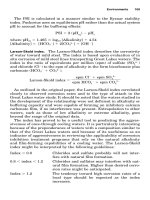
Figure 3.45 compares longitudinal stress distributions obtained by ANSYS with those
by experiments and by the elementary beam theory. The results obtained by three
different methods agree well with one another. As the applied load increases, however,
errors among the three groups of the results become larger, especially at the clamped
end. This tendency arises from the fact that the clamped condition can be hardly
realized in the strict sense.
20 30 40 50 60
Ϫ300
Ϫ200
Ϫ100

0
100
200
300
x-coordinate, x (mm)
Longitudinal stress, σ, (MPa)
100 N
150 N
Pϭ200 N
200 N
150 N
Pϭ100 N
ANSYS
Experiment
Theory
Figure 3.45 Comparison of longitudinal stress distributions obtained by ANSYS with those by experiments
and by the elementary beam theory.
3.1.5
Problems to solve
PROBLEM 3.1
Change the point of load application and the intensity of the applied load in the
cantilever beam model shown in Figure 3.3 and calculate the maximum deflection.
PROBLEM 3.2
Calculate the maximum deflection in a beam clamped at the both ends as shown in
Figure P3.2 where the thickness of the beam in the direction perpendicular to the
page surface is 10 mm.
(Answer: 0.00337 mm)
PROBLEM 3.3
Calculate the maximum deflection in a beam simply supported at the both ends as
shown in Figure P3.3 where the thickness of the beam in the direction perpendicular

to the page surface is 10 mm.
(Answer: 0.00645 mm)
Ch03-H6875.tex 24/11/2006 17: 2 page 77
3.1 Cantilever beam 77
100 mm
100 N
50 mm
10 mm
Figure P3.2 A beam clamped at the both ends and subjected to a concentrated force of 100 N at the center
of the span.
100 mm
100 N
50 mm
10 mm
10 mm
10 mm
Figure P3.3 A beam simply supported at the both ends and subjected to a concentrated force of 100 N at
the center of the span.
PROBLEM 3.4
Calculate the maximum deflection in a beam shown in Figure P3.4 where the thickness
of the beam in the direction perpendicular to the page surface is 10 mm. Choose an
element size of 1 mm.
(Answer: 0.00337 mm)
Note that the beam shown in Figure P3.2 is bilaterally symmetric so that the
x-component of the displacement (DOF X) is zero at the center of the beam span. If
the beam shown in Figure P3.2 is cut at the center of the span and the finite-element
calculation is made for only the left half of the beam by applying a half load of
50 N to its right end which is fixed in the x-direction but is deformed freely in the
y-direction as shown in Figure P3.4, the solution obtained is the same as that for the
left half of the beam in Problem 3.2. Problem 3.2 can be solved by its half model

as shown in Figure P3.4. A half model can achieve the efficiency of finite-element
calculations.
Ch03-H6875.tex 24/11/2006 17: 2 page 78
78 Chapter 3 Application of ANSYS to stress analysis
50 mm
50 N
10 mm
DOF X
Figure P3.4 A half model of the beam in Problem 3.2.
50 mm
50 N
10 mm
10 mm
Figure P3.5 A half model of the beam in Problem 3.3.
PROBLEM 3.5
Calculate the maximum deflection in a beam shown in Figure P3.5 where the thickness
of the beam in the direction perpendicular to the page surface is 10 mm. This beam
is the half model of the beam of Problem 3.3.
(Answer: 0.00645 mm)
PROBLEM 3.6
Calculate the maximum value of the von Mises stress in the stepped beam as shown in
Figure P3.6 where Young’s modulus E =210 GPa, Poisson’s ratio ν =0.3, the element
size is 2 mm and the beam thickness is 10 mm. Refer to the Appendix to create the
stepped beam. The von Mises stress σ
eq
is sometimes called the equivalent stress or
Ch03-H6875.tex 24/11/2006 17: 2 page 79
3.1 Cantilever beam 79
the effective stress and is expressed by the following formula:
σ

eq
=
1
√
2

(σ
x
−σ
y
)
2
+(σ
y
−σ
z
)
2
+(σ
z
−σ
x
)
2
+6(τ
2
xy
+τ
2
yz

+τ
2
zx
) (P3.6)
in three-dimensional elasticity problems. It is often considered that a material yields
when the value of the von Mises stress reaches the yield stress of the material σ
Y
which
is determined by the uniaxial tensile tests of the material.
(Answer: 40.8 MPa)
50 mm
20 mm
10 mm
100 mm
100 N
Figure P3.6 A stepped cantilever beam subjected to a concentrated force of 100 N at the free end.
PROBLEM 3.7
Calculate the maximum value of the von Mises stress in the stepped beam with a
rounded fillet as shown in Figure P3.7 where Young’s modulus E =210 GPa, Pois-
son’s ratio ν =0.3, the element size is 2 mm and the beam thickness is 10 mm. Refer
to the Appendix to create the stepped beam with a rounded fillet.
(Answer: 30.2 MPa)
50 mm
20 mm
10 mm
100 mm
100 N
R10 mm
Figure P3.7 A stepped cantilever beam with a rounded fillet subjected to a concentrated force of 100 N at
the free end.

Ch03-H6875.tex 24/11/2006 17: 2 page 80
80 Chapter 3 Application of ANSYS to stress analysis
A
Figure 3.46 “Add Areas”
window.
Appendix: procedures for
creating stepped beams
A3.1 Creation of a stepped beam
A stepped beam as shown in Figure P3.6 can be
created by adding two rectangular areas of different
sizes:
(1) Create two rectangular areas of different sizes,
say50mmby20mmwithWPX=−50 mm
and WP Y=−10 mm, and 60 mm by 10mm
with WP X=−10 mm and WP Y =−10 mm,
following operations described in 3.1.3.1.
(2) Select the Boolean operation of adding areas
asfollowstoopentheAdd Areas window (see
Figure 3.46)
Command
ANSYS Main Menu →Preprocessor →
Modeling →Operate →Booleans →
Add →Areas
(3) Pick all the areas to add by the upward arrow.
(4) The color of the areas picked turns from light
blue into pink (see Figure 3.47). Click [A] OK
button to add the two rectangular areas to create
a stepped beam area as shown in Figure 3.48.
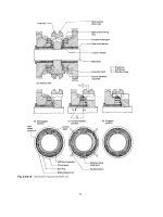
Figure 3.47 Two rectangular areas of different sizes to be added to create a stepped beam area.
Ch03-H6875.tex 24/11/2006 17: 2 page 81

3.1 Cantilever beam 81
Figure 3.48 A stepped beam area created by adding two rectangle areas.
A3.1.1 HOW TO CANCEL THE SELECTION OF AREAS
Click Reset button or click the right button of the mouse to change the upward arrow
to the downward arrow and click the area(s) to pick. The color of the unpicked area(s)
turns pink into light blue and the selection of the area(s) is canceled.
A3.2 Creation of a stepped beam with a rounded fillet
A stepped beam with a rounded fillet as shown in Figure P3.7 can be created by
subtracting a smaller rectangular area and a solid circle from a larger rectangular
area:
(1) Create a larger rectangular area of 100 mm by 20 mm with WP X =−100 mm
and WP Y =−10 mm, a smaller rectangular area of, say 50 mm by 15 mm with
WP X =10 mm and WP Y =0 mm, and a solid circular area having a diameter
of 10 mm with WP X =10 mm and WP Y =10 mm as shown in Figure 3.49. The
solid circular area can be created by executing the following operation:
Command
ANSYS Main Menu →Preprocessor →Modeling →Create →Areas →
Circle →Solid Circle
Ch03-H6875.tex 24/11/2006 17: 2 page 82
82 Chapter 3 Application of ANSYS to stress analysis
Figure 3.49 A larger rectangular area, a smaller rectangular area and a solid circular area to create a stepped
beam area with a rounded fillet.
to open the Solid Circular Area window.
Input the coordinate of the center ([A] WP
X, [B] WP Y) and [C] Radius of the solid
circle and click [D] OK button as shown in
Figure 3.50.
A
B
C

D
Figure 3.50 “Solid Circular Area”
window.
(2) Select the Boolean operation of subtract-
ing areas as follows to open the Subtract
Areas window (see Figure 3.51):
Command
ANSYS Main Menu →Preprocessor →
Modeling →Operate →Booleans →
Subtract →Areas
(3) Pick the larger rectangular area by the
upward arrow as shown in Figure 3.52
and the color of the area picked turns
from light blue into pink. Click [A] OK
button.
(4) Pick the smaller rectangular area and the
solid circular area by the upward arrow
as shown in Figure 3.53 and the color of
the two areas picked turns from light blue
into pink. Click [A] OK button to subtract the smaller rectangular and solid
Ch03-H6875.tex 24/11/2006 17: 2 page 83
A
Figure 3.51 “Subtract Areas”
window.
Figure 3.52 The larger rectangular area picked.
Figure 3.53 The smaller rectangular area and the solid circular area picked to be subtracted from the larger
rectangular area to create a stepped beam area with a rounded fillet.