8. Assessing Product Reliability
8.4. Reliability Data Analysis
8.4.5. How do you fit system repair rate models?
8.4.5.1.Constant repair rate
(HPP/exponential) model
This section
covers
estimating
MTBF's and
calculating
upper and
lower
confidence
bounds
The HPP or exponential model is widely used for two reasons:
Most systems spend most of their useful lifetimes operating in the
flat constant repair rate portion of the bathtub curve
●
It is easy to plan tests, estimate the MTBF and calculate
confidence intervals when assuming the exponential model.
●
This section covers the following:
Estimating the MTBF (or repair rate/failure rate)1.
How to use the MTBF confidence interval factors2.
Tables of MTBF confidence interval factors 3.
Confidence interval equation and "zero fails" case4.
Dataplot/EXCEL calculation of confidence intervals5.
Example6.
Estimating the MTBF (or repair rate/failure rate)
For the HPP system model, as well as for the non repairable exponential
population model, there is only one unknown parameter

(or
equivalently, the MTBF = 1/
). The method used for estimation is the
same for the HPP model and for the exponential population model.
8.4.5.1. Constant repair rate (HPP/exponential) model
(1 of 6) [5/1/2006 10:42:32 AM]
The best
estimate of
the MTBF is
just "Total
Time"
divided by
"Total
Failures"
The estimate of the MTBF is
This estimate is the maximum likelihood estimate whether the data are
censored or complete, or from a repairable system or a non-repairable
population.
Confidence
Interval
Factors
multiply the
estimated
MTBF to
obtain lower
and upper
bounds on
the true
MTBF
How To Use the MTBF Confidence Interval Factors

Estimate the MTBF by the standard estimate (total unit test hours
divided by total failures)
1.
Pick a confidence level (i.e., pick 100x(1-
)). For 95%, = .05;
for 90%,
= .1; for 80%, = .2 and for 60%, = .4
2.
Read off a lower and an upper factor from the confidence interval
tables for the given confidence level and number of failures r
3.
Multiply the MTBF estimate by the lower and upper factors to
obtain MTBF
lower
and MTBF
upper
4.
When r (the number of failures) = 0, multiply the total unit test
hours by the "0 row" lower factor to obtain a 100 × (1-
/2)%
one-sided lower bound for the MTBF. There is no upper bound
when r = 0.
5.
Use (MTBF
lower
, MTBF
upper
) as a 100×(1- )% confidence
interval for the MTBF
(r > 0)

6.
Use MTBF
lower
as a (one-sided) lower 100×(1- /2)% limit for
the MTBF
7.
Use MTBF
upper
as a (one-sided) upper 100×(1- /2)% limit for
the MTBF
8.
Use (1/MTBF
upper
, 1/MTBF
lower
) as a 100×(1- )% confidence
interval for
9.
Use 1/MTBF
upper
as a (one-sided) lower 100×(1- /2)% limit for 10.
8.4.5.1. Constant repair rate (HPP/exponential) model
(2 of 6) [5/1/2006 10:42:32 AM]
Use 1/MTBF
lower
as a (one-sided) upper 100×(1- /2)% limit for 11.
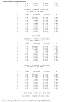
Tables of MTBF Confidence Interval Factors
Confidence
bound factor
tables for

60, 80, 90
and 95%
confidence
Confidence Interval Factors to Multiply MTBF Estimate
60% 80%
Num
Fails r
Lower for
MTBF
Upper for
MTBF
Lower for
MTBF
Upper for
MTBF
0 0.6213 - 0.4343 -
1 0.3340 4.4814 0.2571 9.4912
2 0.4674 2.4260 0.3758 3.7607
3 0.5440 1.9543 0.4490 2.7222
4 0.5952 1.7416 0.5004 2.2926
5 0.6324 1.6184 0.5391 2.0554
6 0.6611 1.5370 0.5697 1.9036
7 0.6841 1.4788 0.5947 1.7974
8 0.7030 1.4347 0.6156 1.7182
9 0.7189 1.4000 0.6335 1.6567
10 0.7326 1.3719 0.6491 1.6074
11 0.7444 1.3485 0.6627 1.5668
12 0.7548 1.3288 0.6749 1.5327
13 0.7641 1.3118 0.6857 1.5036
14 0.7724 1.2970 0.6955 1.4784

15 0.7799 1.2840 0.7045 1.4564
20 0.8088 1.2367 0.7395 1.3769
25 0.8288 1.2063 0.7643 1.3267
30 0.8436 1.1848 0.7830 1.2915
35 0.8552 1.1687 0.7978 1.2652
40 0.8645 1.1560 0.8099 1.2446
45 0.8722 1.1456 0.8200 1.2280
50 0.8788 1.1371 0.8286 1.2142
75 0.9012 1.1090 0.8585 1.1694
100 0.9145 1.0929 0.8766 1.1439
500 0.9614 1.0401 0.9436 1.0603
Confidence Interval Factors to Multiply MTBF Estimate
90% 95%
Num
Fails
Lower for
MTBF
Upper for
MTBF
Lower for
MTBF
Upper for
MTBF
0 0.3338 - 0.2711 -
8.4.5.1. Constant repair rate (HPP/exponential) model
(3 of 6) [5/1/2006 10:42:32 AM]
1 0.2108 19.4958 0.1795 39.4978
2 0.3177 5.6281 0.2768 8.2573
3 0.3869 3.6689 0.3422 4.8491
4 0.4370 2.9276 0.3906 3.6702

5 0.4756 2.5379 0.4285 3.0798
6 0.5067 2.2962 0.4594 2.7249
7 0.5324 2.1307 0.4853 2.4872
8 0.5542 2.0096 0.5075 2.3163
9 0.5731 1.9168 0.5268 2.1869
10 0.5895 1.8432 0.5438 2.0853
11 0.6041 1.7831 0.5589 2.0032
12 0.6172 1.7330 0.5725 1.9353
13 0.6290 1.6906 0.5848 1.8781
14 0.6397 1.6541 0.5960 1.8291
15 0.6494 1.6223 0.6063 1.7867
20 0.6882 1.5089 0.6475 1.6371
25 0.7160 1.4383 0.6774 1.5452
30 0.7373 1.3893 0.7005 1.4822
35 0.7542 1.3529 0.7190 1.4357
40 0.7682 1.3247 0.7344 1.3997
45 0.7800 1.3020 0.7473 1.3710
50 0.7901 1.2832 0.7585 1.3473
75 0.8252 1.2226 0.7978 1.2714
100 0.8469 1.1885 0.8222 1.2290
500 0.9287 1.0781 0.9161 1.0938
Confidence Interval Equation and "Zero Fails" Case
Formulas
for
confidence
bound
factors -
even for
"zero fails"
case

Confidence bounds for the typical Type I censoring situation are
obtained from chi-square distribution tables or programs. The formula
for calculating confidence intervals is:
In this formula, is a value that the chi-square statistic with
2r degrees of freedom is greater than with probability 1-
/2. In other
words, the right-hand tail of the distribution has probability 1-
/2. An
even simpler version of this formula can be written using T = the total
unit test time:
8.4.5.1. Constant repair rate (HPP/exponential) model
(4 of 6) [5/1/2006 10:42:32 AM]
These bounds are exact for the case of one or more repairable systems
on test for a fixed time. They are also exact when non repairable units
are on test for a fixed time and failures are replaced with new units
during the course of the test. For other situations, they are approximate.
When there are zero failures during the test or operation time, only a
(one-sided) MTBF lower bound exists, and this is given by
MTBF
lower
= T/(-ln )
The interpretation of this bound is the following: if the true MTBF were
any lower than MTBF
lower
, we would have seen at least one failure
during T hours of test with probability at least 1-
. Therefore, we are
100×(1-
)% confident that the true MTBF is not lower than
MTBF

lower
.
Dataplot/EXCEL Calculation of Confidence Intervals
Dataplot
and EXCEL
calculation
of
confidence
limits
A lower 100×(1-
/2)% confidence bound for the MTBF is given by
LET LOWER = T*2/CHSPPF( [1-
/2], [2*(r+1)])
where T is the total unit or system test time and r is the total number of
failures.
The upper 100×(1-
/2)% confidence bound is
LET UPPER = T*2/CHSPPF(
/2,[2*r])
and (LOWER, UPPER) is a 100× (1-
) confidence interval for the true
MTBF.
The same calculations can be performed with EXCEL built-in functions
with the commands
=T*2/CHIINV([ /2], [2*(r+1)]) for the lower bound and
=T*2/CHIINV( [1-
/2],[2*r]) for the upper bound.
Note that the Dataplot CHSPPF function requires left tail probability
inputs (i.e., /2 for the lower bound and 1- /2 for the upper bound),
while the EXCEL CHIINV function requires right tail inputs (i.e., 1-

/2 for the lower bound and /2 for the upper bound).
Example
8.4.5.1. Constant repair rate (HPP/exponential) model
(5 of 6) [5/1/2006 10:42:32 AM]
Example
showing
how to
calculate
confidence
limits
A system was observed for two calendar months of operation, during
which time it was in operation for 800 hours and had 2 failures.
The MTBF estimate is 800/2 = 400 hours. A 90% confidence interval is
given by (400×.3177, 400×5.6281) = (127, 2251). The same interval
could have been obtained using the Dataplot commands
LET LOWER = 1600/CHSPPF(.95,6)
LET UPPER = 1600/CHSPPF(.05,4)
or the EXCEL commands
=1600/CHIINV(.05,6) for the lower limit
=1600/CHIINV(.95,4) for the upper limit.
Note that 127 is a 95% lower limit for the true MTBF. The customer is
usually only concerned with the lower limit and one-sided lower limits
are often used for statements of contractual requirements.
Zero fails
confidence
limit
calculation
What could we have said if the system had no failures? For a 95% lower
confidence limit on the true MTBF, we either use the 0 failures factor
from the 90% confidence interval table and calculate 800 × .3338 = 267

or we use T/(
-ln ) = 800/(-ln.05) = 267.
8.4.5.1. Constant repair rate (HPP/exponential) model
(6 of 6) [5/1/2006 10:42:32 AM]
The estimated MTBF at the end of the test (or observation) period is
Approximate
confidence
bounds for
the MTBF at
end of test
are given
Approximate Confidence Bounds for the MTBF at End of Test
We give an approximate 100×(1-
)% confidence interval (M
L
, M
U
)
for the MTBF at the end of the test. Note that M
L
is a 100×(1- /2)%
lower bound and M
U
is a 100×(1- /2)% upper bound. The formulas
are:
with is the upper 100×(1- /2) percentile point of the standard
normal distribution.

8.4.5.2. Power law (Duane) model
(2 of 3) [5/1/2006 10:42:34 AM]

Dataplot
calculations
for the
Power Law
(Duane)
Model
Dataplot Estimates And Confidence Bounds For the Power Law
Model
Dataplot will calculate
, a, and the MTBF at the end of test, along
with a 100x(1-
)% confidence interval for the true MTBF at the end of
test (assuming, of course, that the Power Law model holds). The user
needs to pull down the Reliability menu and select "Test" and "Power
Law Model". The times of failure can be entered on the Dataplot spread
sheet. A Dataplot example is shown next.
Case Study 1: Reliability Improvement Test Data Continued
Dataplot
results
fitting the
Power Law
model to
Case Study
1 failure
data
This case study was introduced in section 2, where we did various plots
of the data, including a Duane Plot. The case study was continued when
we discussed trend tests and verified that significant improvement had
taken place. Now we will use Dataplot to complete the case study data
analysis.

The observed failure times were: 5, 40, 43, 175, 389, 712, 747, 795,
1299 and 1478 hours, with the test ending at 1500 hours. After entering
this information into the "Reliability/Test/Power Law Model" screen
and the Dataplot spreadsheet and selecting a significance level of .2 (for
an 80% confidence level), Dataplot gives the following output:
THE RELIABILITY GROWTH SLOPE BETA IS 0.516495
THE A PARAMETER IS 0.2913
THE MTBF AT END OF TEST IS 310.234
THE DESIRED 80 PERCENT CONFIDENCE INTERVAL IS:
(157.7139 , 548.5565)
AND 157.7139 IS A (ONE-SIDED) 90 PERCENT
LOWER LIMIT
Note: The downloadable package of statistical programs, SEMSTAT,
will also calculate Power Law model statistics and construct Duane
plots. The routines are reached by selecting "Reliability" from the main
menu then the "Exponential Distribution" and finally "Duane
Analysis".
8.4.5.2. Power law (Duane) model
(3 of 3) [5/1/2006 10:42:34 AM]
8.4.5.3. Exponential law model
(2 of 2) [5/1/2006 10:42:34 AM]
How to
estimate
the MTBF
with
bounds,
based on
the
posterior
distribution

Once the test has been run, and r failures observed, the posterior gamma parameters are:
a' = a + r, b' = b + T
and a (median) estimate for the MTBF, using EXCEL, is calculated by
= 1/GAMMAINV(.5, a', (1/ b'))
Some people prefer to use the reciprocal of the mean of the posterior distribution as their estimate
for the MTBF. The mean is the minimum mean square error (MSE) estimator of
, but using
the reciprocal of the mean to estimate the MTBF is always more conservative than the "even
money" 50% estimator.
A lower 80% bound for the MTBF is obtained from
= 1/GAMMAINV(.8, a', (1/ b'))
and, in general, a lower 100×(1-
)% lower bound is given by
= 1/GAMMAINV((1-
), a', (1/ b')).
A two sided 100× (1-
)% credibility interval for the MTBF is
[{= 1/GAMMAINV((1-
/2), a', (1/ b'))},{= 1/GAMMAINV(( /2), a', (1/ b'))}].
Finally, = GAMMADIST((1/M), a', (1/b'), TRUE) calculates the probability the MTBF is greater
than M.
Example
A Bayesian
example
using
EXCEL to
estimate
the MTBF
and
calculate

upper and
lower
bounds
A system has completed a reliability test aimed at confirming a 600 hour MTBF at an 80%
confidence level. Before the test, a gamma prior with a = 2, b = 1400 was agreed upon, based on
testing at the vendor's location. Bayesian test planning calculations, allowing up to 2 new failures,
called for a test of 1909 hours. When that test was run, there actually were exactly two failures.
What can be said about the system?
The posterior gamma CDF has parameters a' = 4 and b' = 3309. The plot below shows CDF
values on the y-axis, plotted against 1/
= MTBF, on the x-axis. By going from probability, on
the y-axis, across to the curve and down to the MTBF, we can read off any MTBF percentile
point we want. (The EXCEL formulas above will give more accurate MTBF percentile values
than can be read off a graph.)
8.4.6. How do you estimate reliability using the Bayesian gamma prior model?
(2 of 3) [5/1/2006 10:42:35 AM]
The MTBF values are shown below:
= 1/GAMMAINV(.9, 4, (1/ 3309)) has value 495 hours
= 1/GAMMAINV(.8, 4, (1/ 3309)) has value 600 hours (as expected)
= 1/GAMMAINV(.5, 4, (1/ 3309)) has value 901 hours
= 1/GAMMAINV(.1, 4, (1/ 3309)) has value 1897 hours
The test has confirmed a 600 hour MTBF at 80% confidence, a 495 hour MTBF at 90 %
confidence and (495, 1897) is a 90 percent credibility interval for the MTBF. A single number
(point) estimate for the system MTBF would be 901 hours. Alternatively, you might want to use
the reciprocal of the mean of the posterior distribution (b'/a') = 3309/4 = 827 hours as a single
estimate. The reciprocal mean is more conservative
- in this case it is a 57% lower bound, as
=GAMMADIST((4/3309),4,(1/3309),TRUE) shows.
8.4.6. How do you estimate reliability using the Bayesian gamma prior model?
(3 of 3) [5/1/2006 10:42:35 AM]

Crow, L.H. (1990), "Evaluating the Reliability of Repairable Systems," Proceedings
Annual Reliability and Maintainability Symposium, pp. 275-279.
Crow, L.H. (1993), "Confidence Intervals on the Reliability of Repairable Systems,"
Proceedings Annual Reliability and Maintainability Symposium, pp. 126-134
Duane, J.T. (1964), "Learning Curve Approach to Reliability Monitoring," IEEE
Transactions On Aerospace, 2, pp. 563-566.
Gumbel, E. J. (1954), Statistical Theory of Extreme Values and Some Practical
Applications, National Bureau of Standards Applied Mathematics Series 33, U.S.
Government Printing Office, Washington, D.C.
Hahn, G.J., and Shapiro, S.S. (1967), Statistical Models in Engineering, John Wiley &
Sons, Inc., New York.
Hoyland, A., and Rausand, M. (1994), System Reliability Theory, John Wiley & Sons,
Inc., New York.
Johnson, N.L., Kotz, S. and Balakrishnan, N. (1994), Continuous Univariate
Distributions Volume 1, 2nd edition, John Wiley & Sons, Inc., New York.
Johnson, N.L., Kotz, S. and Balakrishnan, N. (1995), Continuous Univariate
Distributions Volume 2, 2nd edition, John Wiley & Sons, Inc., New York.
Kaplan, E.L., and Meier, P. (1958), "Nonparametric Estimation From Incomplete
Observations," Journal of the American Statistical Association, 53: 457-481.
Kalbfleisch, J.D., and Prentice, R.L. (1980), The Statistical Analysis of Failure Data,
John Wiley & Sons, Inc., New York.
Kielpinski, T.J., and Nelson, W.(1975), "Optimum Accelerated Life-Tests for the
Normal and Lognormal Life Distributins," IEEE Transactions on Reliability, Vol. R-24,
5, pp. 310-320.
Klinger, D.J., Nakada, Y., and Menendez, M.A. (1990), AT&T Reliability Manual, Van
Nostrand Reinhold, Inc, New York.
Kolmogorov, A.N. (1941), "On A Logarithmic Normal Distribution Law Of The
Dimensions Of Particles Under Pulverization," Dokl. Akad Nauk, USSR 31, 2, pp.
99-101.
Kovalenko, I.N., Kuznetsov, N.Y., and Pegg, P.A. (1997), Mathematical Theory of

Reliability of Time Dependent Systems with Practical Applications, John Wiley & Sons,
Inc., New York.
Landzberg, A.H., and Norris, K.C. (1969), "Reliability of Controlled Collapse
Interconnections." IBM Journal Of Research and Development, Vol. 13, 3.
Lawless, J.F. (1982), Statistical Models and Methods For Lifetime Data, John Wiley &
8.4.7. References For Chapter 8: Assessing Product Reliability
(2 of 4) [5/1/2006 10:42:41 AM]
Sons, Inc., New York.
Leon, R. (1997-1999), JMP Statistical Tutorials on the Web at
/>Mann, N.R., Schafer, R.E. and Singpurwalla, N.D. (1974), Methods For Statistical
Analysis Of Reliability & Life Data, John Wiley & Sons, Inc., New York.
Martz, H.F., and Waller, R.A. (1982), Bayesian Reliability Analysis, Krieger Publishing
Company, Malabar, Florida.
Meeker, W.Q., and Escobar, L.A. (1998), Statistical Methods for Reliability Data, John
Wiley & Sons, Inc., New York.
Meeker, W.Q., and Hahn, G.J. (1985), "How to Plan an Accelerated Life Test - Some
Practical Guidelines," ASC Basic References In Quality Control: Statistical Techniques -
Vol. 10, ASQC , Milwaukee, Wisconsin.
Meeker, W.Q., and Nelson, W. (1975), "Optimum Accelerated Life-Tests for the
Weibull and Extreme Value Distributions," IEEE Transactions on Reliability, Vol. R-24,
5, pp. 321-322.
Michael, J.R., and Schucany, W.R. (1986), "Analysis of Data From Censored Samples,"
Goodness of Fit Techniques, ed. by D'Agostino, R.B., and Stephens, M.A., Marcel
Dekker, New York.
MIL-HDBK-189 (1981), Reliability Growth Management, U.S. Government Printing
Office.
MIL-HDBK-217F ((1986), Reliability Prediction of Electronic Equipment, U.S.
Government Printing Office.
MIL-STD-1635 (EC) (1978), Reliability Growth Testing, U.S. Government Printing
Office.

Nelson, W. (1990), Accelerated Testing, John Wiley & Sons, Inc., New York.
Nelson, W. (1982), Applied Life Data Analysis, John Wiley & Sons, Inc., New York.
O'Connor, P.D.T. (1991), Practical Reliability Engineering (Third Edition), John Wiley
& Sons, Inc., New York.
Peck, D., and Trapp, O.D. (1980), Accelerated Testing Handbook, Technology
Associates and Bell Telephone Laboratories, Portola, Calif.
Pore, M., and Tobias, P. (1998), "How Exact are 'Exact' Exponential System MTBF
Confidence Bounds?", 1998 Proceedings of the Section on Physical and Engineering
Sciences of the American Statistical Association.
SEMI E10-0701, (2001), Standard For Definition and Measurement of Equipment
Reliability, Availability and Maintainability (RAM), Semiconductor Equipment and
Materials International, Mountainview, CA.
8.4.7. References For Chapter 8: Assessing Product Reliability
(3 of 4) [5/1/2006 10:42:41 AM]
Tobias, P. A., and Trindade, D. C. (1995), Applied Reliability, 2nd edition, Chapman and
Hall, London, New York.

8.4.7. References For Chapter 8: Assessing Product Reliability
(4 of 4) [5/1/2006 10:42:41 AM]