6. Process or Product Monitoring and Control
6.4. Introduction to Time Series Analysis
6.4.4. Univariate Time Series Models
6.4.4.3.Seasonality
Seasonality Many time series display seasonality. By seasonality, we mean periodic
fluctuations. For example, retail sales tend to peak for the Christmas
season and then decline after the holidays. So time series of retail sales
will typically show increasing sales from September through December
and declining sales in January and February.
Seasonality is quite common in economic time series. It is less common
in engineering and scientific data.
If seasonality is present, it must be incorporated into the time series
model. In this section, we discuss techniques for detecting seasonality.
We defer modeling of seasonality until later sections.
Detecting
Seasonality
he following graphical techniques can be used to detect seasonality.
A run sequence plot will often show seasonality.1.
A seasonal subseries plot is a specialized technique for showing
seasonality.
2.
Multiple box plots can be used as an alternative to the seasonal
subseries plot to detect seasonality.
3.
The autocorrelation plot can help identify seasonality.4.
Examples of each of these plots will be shown below.
The run sequence plot is a recommended first step for analyzing any
time series. Although seasonality can sometimes be indicated with this
plot, seasonality is shown more clearly by the seasonal subseries plot or
the box plot. The seasonal subseries plot does an excellent job of
showing both the seasonal differences (between group patterns) and also

the within-group patterns. The box plot shows the seasonal difference
(between group patterns) quite well, but it does not show within group
patterns. However, for large data sets, the box plot is usually easier to
read than the seasonal subseries plot.
Both the seasonal subseries plot and the box plot assume that the
6.4.4.3. Seasonality
(1 of 5) [5/1/2006 10:35:20 AM]
seasonal periods are known. In most cases, the analyst will in fact know
this. For example, for monthly data, the period is 12 since there are 12
months in a year. However, if the period is not known, the
autocorrelation plot can help. If there is significant seasonality, the
autocorrelation plot should show spikes at lags equal to the period. For
example, for monthly data, if there is a seasonality effect, we would
expect to see significant peaks at lag 12, 24, 36, and so on (although the
intensity may decrease the further out we go).
Example
without
Seasonality
The following plots are from a data set of southern oscillations for
predicting el nino.
Run
Sequence
Plot
No obvious periodic patterns are apparent in the run sequence plot.
6.4.4.3. Seasonality
(2 of 5) [5/1/2006 10:35:20 AM]
Seasonal
Subseries
Plot
The means for each month are relatively close and show no obvious

pattern.
Box Plot
As with the seasonal subseries plot, no obvious seasonal pattern is
apparent.
Due to the rather large number of observations, the box plot shows the
difference between months better than the seasonal subseries plot.
6.4.4.3. Seasonality
(3 of 5) [5/1/2006 10:35:20 AM]
Example
with
Seasonality
The following plots are from a data set of monthly CO2 concentrations.
A linear trend has been removed from these data.
Run
Sequence
Plot
This plot shows periodic behavior. However, it is difficult to determine
the nature of the seasonality from this plot.
Seasonal
Subseries
Plot
The seasonal subseries plot shows the seasonal pattern more clearly. In
6.4.4.3. Seasonality
(4 of 5) [5/1/2006 10:35:20 AM]
this case, the CO
2
concentrations are at a minimun in September and
October. From there, steadily the concentrations increase until June and
then begin declining until September.
Box Plot

As with the seasonal subseries plot, the seasonal pattern is quite evident
in the box plot.
6.4.4.3. Seasonality
(5 of 5) [5/1/2006 10:35:20 AM]
This plot allows you to detect both between group and within group
patterns.
If there is a large number of observations, then a box plot may be
preferable.
Definition Seasonal subseries plots are formed by
Vertical axis: Response variable
Horizontal axis: Time ordered by season. For example, with
monthly data, all the January values are plotted
(in chronological order), then all the February
values, and so on.
In addition, a reference line is drawn at the group means.
The user must specify the length of the seasonal pattern before
generating this plot. In most cases, the analyst will know this from the
context of the problem and data collection.
Questions The seasonal subseries plot can provide answers to the following
questions:
Do the data exhibit a seasonal pattern?1.
What is the nature of the seasonality?2.
Is there a within-group pattern (e.g., do January and July exhibit
similar patterns)?
3.
Are there any outliers once seasonality has been accounted for?4.
Importance It is important to know when analyzing a time series if there is a
significant seasonality effect. The seasonal subseries plot is an excellent
tool for determining if there is a seasonal pattern.
Related

Techniques
Box Plot
Run Sequence Plot
Autocorrelation Plot
Software Seasonal subseries plots are available in a few general purpose statistical
software programs. They are available in Dataplot. It may possible to
write macros to generate this plot in most statistical software programs
that do not provide it directly.
6.4.4.3.1. Seasonal Subseries Plot
(2 of 2) [5/1/2006 10:35:20 AM]
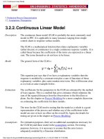
Autoregressive
(AR) Models
A common approach for modeling univariate time series is the
autoregressive (AR) model:
where X
t
is the time series, A
t
is white noise, and
with denoting the process mean.
An autoregressive model is simply a linear regression of the current
value of the series against one or more prior values of the series. The
value of p is called the order of the AR model.
AR models can be analyzed with one of various methods, including
standard linear least squares techniques. They also have a
straightforward interpretation.
Moving
Average (MA)
Models
Another common approach for modeling univariate time series

models is the moving average (MA) model:
where X
t
is the time series, is the mean of the series, A
t-i
are white
noise, and
1
, ,
q
are the parameters of the model. The value of q
is called the order of the MA model.
That is, a moving average model is conceptually a linear regression of
the current value of the series against the white noise or random
shocks of one or more prior values of the series. The random shocks
at each point are assumed to come from the same distribution,
typically a normal distribution, with location at zero and constant
scale. The distinction in this model is that these random shocks are
propogated to future values of the time series. Fitting the MA
estimates is more complicated than with AR models because the error
terms are not observable. This means that iterative non-linear fitting
procedures need to be used in place of linear least squares. MA
models also have a less obvious interpretation than AR models.
Sometimes the ACF and PACF will suggest that a MA model would
be a better model choice and sometimes both AR and MA terms
should be used in the same model (see Section 6.4.4.5).
Note, however, that the error terms after the model is fit should be
independent and follow the standard assumptions for a univariate
process.
6.4.4.4. Common Approaches to Univariate Time Series

(2 of 3) [5/1/2006 10:35:21 AM]
Box-Jenkins
Approach
Box and Jenkins popularized an approach that combines the moving
average and the autoregressive approaches in the book "Time Series
Analysis: Forecasting and Control" (Box, Jenkins, and Reinsel,
1994).
Although both autoregressive and moving average approaches were
already known (and were originally investigated by Yule), the
contribution of Box and Jenkins was in developing a systematic
methodology for identifying and estimating models that could
incorporate both approaches. This makes Box-Jenkins models a
powerful class of models. The next several sections will discuss these
models in detail.
6.4.4.4. Common Approaches to Univariate Time Series
(3 of 3) [5/1/2006 10:35:21 AM]
Stages in
Box-Jenkins
Modeling
There are three primary stages in building a Box-Jenkins time series
model.
Model Identification1.
Model Estimation2.
Model Validation3.
Remarks The following remarks regarding Box-Jenkins models should be noted.
Box-Jenkins models are quite flexible due to the inclusion of both
autoregressive and moving average terms.
1.
Based on the Wold decomposition thereom (not discussed in the
Handbook), a stationary process can be approximated by an

ARMA model. In practice, finding that approximation may not be
easy.
2.
Chatfield (1996) recommends decomposition methods for series
in which the trend and seasonal components are dominant.
3.
Building good ARIMA models generally requires more
experience than commonly used statistical methods such as
regression.
4.
Sufficiently
Long Series
Required
Typically, effective fitting of Box-Jenkins models requires at least a
moderately long series. Chatfield (1996) recommends at least 50
observations. Many others would recommend at least 100 observations.
6.4.4.5. Box-Jenkins Models
(2 of 2) [5/1/2006 10:35:21 AM]
Identify p and q Once stationarity and seasonality have been addressed, the next step
is to identify the order (i.e., the p and q) of the autoregressive and
moving average terms.
Autocorrelation
and Partial
Autocorrelation
Plots
The primary tools for doing this are the autocorrelation plot and the
partial autocorrelation plot. The sample autocorrelation plot and the
sample partial autocorrelation plot are compared to the theoretical
behavior of these plots when the order is known.
Order of

Autoregressive
Process (p)
Specifically, for an AR(1) process, the sample autocorrelation
function should have an exponentially decreasing appearance.
However, higher-order AR processes are often a mixture of
exponentially decreasing and damped sinusoidal components.
For higher-order autoregressive processes, the sample autocorrelation
needs to be supplemented with a partial autocorrelation plot. The
partial autocorrelation of an AR(p) process becomes zero at lag p+1
and greater, so we examine the sample partial autocorrelation
function to see if there is evidence of a departure from zero. This is
usually determined by placing a 95% confidence interval on the
sample partial autocorrelation plot (most software programs that
generate sample autocorrelation plots will also plot this confidence
interval). If the software program does not generate the confidence
band, it is approximately
, with N denoting the sample
size.
Order of
Moving
Average
Process (q)
The autocorrelation function of a MA(q) process becomes zero at lag
q+1 and greater, so we examine the sample autocorrelation function
to see where it essentially becomes zero. We do this by placing the
95% confidence interval for the sample autocorrelation function on
the sample autocorrelation plot. Most software that can generate the
autocorrelation plot can also generate this confidence interval.
The sample partial autocorrelation function is generally not helpful
for identifying the order of the moving average process.

6.4.4.6. Box-Jenkins Model Identification
(2 of 4) [5/1/2006 10:35:27 AM]
Shape of
Autocorrelation
Function
The following table summarizes how we use the sample
autocorrelation function for model identification.
SHAPE INDICATED MODEL
Exponential, decaying to
zero
Autoregressive model. Use the
partial autocorrelation plot to
identify the order of the
autoregressive model.
Alternating positive and
negative, decaying to
zero
Autoregressive model. Use the
partial autocorrelation plot to
help identify the order.
One or more spikes, rest
are essentially zero
Moving average model, order
identified by where plot
becomes zero.
Decay, starting after a
few lags
Mixed autoregressive and
moving average model.
All zero or close to zero Data is essentially random.

High values at fixed
intervals
Include seasonal
autoregressive term.
No decay to zero Series is not stationary.
Mixed Models
Difficult to
Identify
In practice, the sample autocorrelation and partial autocorrelation
functions are random variables and will not give the same picture as
the theoretical functions. This makes the model identification more
difficult. In particular, mixed models can be particularly difficult to
identify.
Although experience is helpful, developing good models using these
sample plots can involve much trial and error. For this reason, in
recent years information-based criteria such as FPE (Final Prediction
Error) and AIC (Aikake Information Criterion) and others have been
preferred and used. These techniques can help automate the model
identification process. These techniques require computer software to
use. Fortunately, these techniques are available in many commerical
statistical software programs that provide ARIMA modeling
capabilities.
For additional information on these techniques, see Brockwell and
Davis (1987, 2002).
6.4.4.6. Box-Jenkins Model Identification
(3 of 4) [5/1/2006 10:35:27 AM]
Examples We show a typical series of plots for performing the initial model
identification for
the southern oscillations data and1.
the CO

2
monthly concentrations data.2.
6.4.4.6. Box-Jenkins Model Identification
(4 of 4) [5/1/2006 10:35:27 AM]
Seasonal
Subseries Plot
The seasonal subseries plot indicates that there is no significant
seasonality.
Since the above plots show that this series does not exhibit any
significant non-stationarity or seasonality, we generate the
autocorrelation and partial autocorrelation plots of the raw data.
Autocorrelation
Plot
The autocorrelation plot shows a mixture of exponentially decaying
6.4.4.6.1. Model Identification for Southern Oscillations Data
(2 of 3) [5/1/2006 10:35:28 AM]
and damped sinusoidal components. This indicates that an
autoregressive model, with order greater than one, may be
appropriate for these data. The partial autocorrelation plot should be
examined to determine the order.
Partial
Autocorrelation
Plot
The partial autocorrelation plot suggests that an AR(2) model might
be appropriate.
In summary, our intial attempt would be to fit an AR(2) model with
no seasonal terms and no differencing or trend removal. Model
validation should be performed before accepting this as a final
model.
6.4.4.6.1. Model Identification for Southern Oscillations Data

(3 of 3) [5/1/2006 10:35:28 AM]