Example Let us illustrate this principle with an example. Consider the following
data set consisting of 12 observations taken over time:
Time
y
t
S ( =.1) Error
Error
squared
1 71
2 70 71 -1.00 1.00
3 69 70.9 -1.90 3.61
4 68 70.71 -2.71 7.34
5 64 70.44 -6.44 41.47
6 65 69.80 -4.80 23.04
7 72 69.32 2.68 7.18
8 78 69.58 8.42 70.90
9 75 70.43 4.57 20.88
10 75 70.88 4.12 16.97
11 75 71.29 3.71 13.76
12 70 71.67 -1.67 2.79
The sum of the squared errors (SSE) = 208.94. The mean of the squared
errors (MSE) is the SSE /11 = 19.0.
Calculate
for different
values of
The MSE was again calculated for = .5 and turned out to be 16.29, so
in this case we would prefer an
of .5. Can we do better? We could
apply the proven trial-and-error method. This is an iterative procedure
beginning with a range of
between .1 and .9. We determine the best

initial choice for
and then search between - and + . We
could repeat this perhaps one more time to find the best
to 3 decimal
places.
Nonlinear
optimizers
can be used
But there are better search methods, such as the Marquardt procedure.
This is a nonlinear optimizer that minimizes the sum of squares of
residuals. In general, most well designed statistical software programs
should be able to find the value of
that minimizes the MSE.
6.4.3.1. Single Exponential Smoothing
(4 of 5) [5/1/2006 10:35:10 AM]
Sample plot
showing
smoothed
data for 2
values of
6.4.3.1. Single Exponential Smoothing
(5 of 5) [5/1/2006 10:35:10 AM]
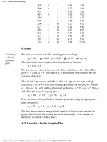
Example of Bootstrapping
Example The last data point in the previous example was 70 and its forecast
(smoothed value S) was 71.7. Since we do have the data point and the
forecast available, we can calculate the next forecast using the regular
formula
= .1(70) + .9(71.7) = 71.5 ( = .1)
But for the next forecast we have no data point (observation). So now
we compute:

S
t+2
=. 1(70) + .9(71.5 )= 71.35
Comparison between bootstrap and regular forecasting
Table
comparing
two methods
The following table displays the comparison between the two methods:
Period Bootstrap
forecast
Data Single Smoothing
Forecast
13 71.50 75 71.5
14 71.35 75 71.9
15 71.21 74 72.2
16 71.09 78 72.4
17 70.98 86 73.0
Single Exponential Smoothing with Trend
Single Smoothing (short for single exponential smoothing) is not very
good when there is a trend. The single coefficient
is not enough.
6.4.3.2. Forecasting with Single Exponential Smoothing
(2 of 3) [5/1/2006 10:35:13 AM]
Sample data
set with trend
Let us demonstrate this with the following data set smoothed with an
of 0.3:
Data Fit
6.4
5.6 6.4

7.8 6.2
8.8 6.7
11.0 7.3
11.6 8.4
16.7 9.4
15.3 11.6
21.6 12.7
22.4 15.4
Plot
demonstrating
inadequacy of
single
exponential
smoothing
when there is
trend
The resulting graph looks like:
6.4.3.2. Forecasting with Single Exponential Smoothing
(3 of 3) [5/1/2006 10:35:13 AM]
Meaning of
the
smoothing
equations
The first smoothing equation adjusts S
t
directly for the trend of the
previous period, b
t-1
, by adding it to the last smoothed value, S
t-1

. This
helps to eliminate the lag and brings S
t
to the appropriate base of the
current value.
The second smoothing equation then updates the trend, which is
expressed as the difference between the last two values. The equation is
similar to the basic form of single smoothing, but here applied to the
updating of the trend.
Non-linear
optimization
techniques
can be used
The values for
and can be obtained via non-linear optimization
techniques, such as the Marquardt Algorithm.
6.4.3.3. Double Exponential Smoothing
(2 of 2) [5/1/2006 10:35:14 AM]
Forecasting
results for
the example
The smoothed results for the example are:
Data Double Single
6.4 6.4
5.6 6.6 (Forecast = 7.2) 6.4
7.8 7.2 (Forecast = 6.8) 5.6
8.8 8.1 (Forecast = 7.8) 7.8
11.0 9.8 (Forecast = 9.1) 8.8
11.6 11.5 (Forecast = 11.4) 10.9
16.7 14.5 (Forecast = 13.2) 11.6

15.3 16.7 (Forecast = 17.4) 16.6
21.6 19.9 (Forecast = 18.9) 15.3
22.4 22.8 (Forecast = 23.1) 21.5
Comparison of Forecasts
Table
showing
single and
double
exponential
smoothing
forecasts
To see how each method predicts the future, we computed the first five
forecasts from the last observation as follows:
Period Single Double
11 22.4 25.8
12 22.4 28.7
13 22.4 31.7
14 22.4 34.6
15 22.4 37.6
Plot
comparing
single and
double
exponential
smoothing
forecasts
A plot of these results (using the forecasted double smoothing values) is
very enlightening.
6.4.3.4. Forecasting with Double Exponential Smoothing(LASP)
(2 of 4) [5/1/2006 10:35:15 AM]

This graph indicates that double smoothing follows the data much closer
than single smoothing. Furthermore, for forecasting single smoothing
cannot do better than projecting a straight horizontal line, which is not
very likely to occur in reality. So in this case double smoothing is
preferred.
Plot
comparing
double
exponential
smoothing
and
regression
forecasts
Finally, let us compare double smoothing with linear regression:
This is an interesting picture. Both techniques follow the data in similar
fashion, but the regression line is more conservative. That is, there is a
slower increase with the regression line than with double smoothing.
6.4.3.4. Forecasting with Double Exponential Smoothing(LASP)
(3 of 4) [5/1/2006 10:35:15 AM]
Selection of
technique
depends on
the
forecaster
The selection of the technique depends on the forecaster. If it is desired
to portray the growth process in a more aggressive manner, then one
selects double smoothing. Otherwise, regression may be preferable. It
should be noted that in linear regression "time" functions as the
independent variable. Chapter 4 discusses the basics of linear regression,
and the details of regression estimation.

6.4.3.4. Forecasting with Double Exponential Smoothing(LASP)
(4 of 4) [5/1/2006 10:35:15 AM]
Complete
season
needed
To initialize the HW method we need at least one complete season's data to
determine initial estimates of the seasonal indices I
t-L
.
L periods
in a season
A complete season's data consists of L periods. And we need to estimate the
trend factor from one period to the next. To accomplish this, it is advisable
to use two complete seasons; that is, 2L periods.
Initial values for the trend factor
How to get
initial
estimates
for trend
and
seasonality
parameters
The general formula to estimate the initial trend is given by
Initial values for the Seasonal Indices
As we will see in the example, we work with data that consist of 6 years
with 4 periods (that is, 4 quarters) per year. Then
Step 1:
compute
yearly
averages

Step 1: Compute the averages of each of the 6 years
Step 2:
divide by
yearly
averages
Step 2: Divide the observations by the appropriate yearly mean
1 2 3 4 5 6
y
1
/A
1
y
5
/A
2
y
9
/A
3
y
13
/A
4
y
17
/A
5
y
21
/A

6
y
2
/A
1
y
6
/A
2
y
10
/A
3
y
14
/A
4
y
18
/A
5
y
22
/A
6
y
3
/A
1
y

7
/A
2
y
11
/A
3
y
15
/A
4
y
19
/A
5
y
23
/A
6
y
4
/A
1
y
8
/A
2
y
12
/A

3
y
16
/A
4
y
20
/A
5
y
24
/A
6
6.4.3.5. Triple Exponential Smoothing
(2 of 3) [5/1/2006 10:35:16 AM]
Step 3:
form
seasonal
indices
Step 3: Now the seasonal indices are formed by computing the average of
each row. Thus the initial seasonal indices (symbolically) are:
I
1
= ( y
1
/A
1
+ y
5
/A

2
+ y
9
/A
3
+ y
13
/A
4
+ y
17
/A
5
+ y
21
/A
6
)/6
I
2
= ( y
2
/A
1
+ y
6
/A
2
+ y
10

/A
3
+ y
14
/A
4
+ y
18
/A
5
+ y
22
/A
6
)/6
I
3
= ( y
3
/A
1
+ y
7
/A
2
+ y
11
/A
3
+ y

15
/A
4
+ y
19
/A
5
+ y
22
/A
6
)/6
I
4
= ( y
4
/A
1
+ y
8
/A
2
+ y
12
/A
3
+ y
16
/A
4

+ y
20
/A
5
+ y
24
/A
6
)/6
We now know the algebra behind the computation of the initial estimates.
The next page contains an example of triple exponential smoothing.
The case of the Zero Coefficients
Zero
coefficients
for trend
and
seasonality
parameters
Sometimes it happens that a computer program for triple exponential
smoothing outputs a final coefficient for trend (
) or for seasonality ( ) of
zero. Or worse, both are outputted as zero!
Does this indicate that there is no trend and/or no seasonality?
Of course not! It only means that the initial values for trend and/or
seasonality were right on the money. No updating was necessary in order to
arrive at the lowest possible MSE. We should inspect the updating formulas
to verify this.
6.4.3.5. Triple Exponential Smoothing
(3 of 3) [5/1/2006 10:35:16 AM]
Plot of raw

data with
single,
double, and
triple
exponential
forecasts
Plot of raw
data with
triple
exponential
forecasts
Actual Time Series with forecasts
6.4.3.6. Example of Triple Exponential Smoothing
(2 of 3) [5/1/2006 10:35:17 AM]
Comparison
of MSE's
Comparison of MSE's
MSE demand trend seasonality
6906 .4694
5054 .1086 1.000
936 1.000 1.000
520 .7556 0.000 .9837
The updating coefficients were chosen by a computer program such that
the MSE for each of the methods was minimized.
Example of the computation of the Initial Trend
Computation
of initial
trend
The data set consists of quarterly sales data. The season is 1 year and
since there are 4 quarters per year, L = 4. Using the formula we obtain:

Example of the computation of the Initial Seasonal Indices
Table of
initial
seasonal
indices
1 2 3 4 5 6
1 362 382 473 544 628 627
2 385 409 513 582 707 725
3 432 498 582 681 773 854
4 341 387 474 557 592 661
380 419 510.5 591 675 716.75
In this example we used the full 6 years of data. Other schemes may use
only 3, or some other number of years. There are also a number of ways
to compute initial estimates.
6.4.3.6. Example of Triple Exponential Smoothing
(3 of 3) [5/1/2006 10:35:17 AM]
6. Process or Product Monitoring and Control
6.4. Introduction to Time Series Analysis
6.4.4.Univariate Time Series Models
Univariate
Time Series
The term "univariate time series" refers to a time series that consists of
single (scalar) observations recorded sequentially over equal time
increments. Some examples are monthly CO
2
concentrations and
southern oscillations to predict el nino effects.
Although a univariate time series data set is usually given as a single
column of numbers, time is in fact an implicit variable in the time series.
If the data are equi-spaced, the time variable, or index, does not need to

be explicitly given. The time variable may sometimes be explicitly used
for plotting the series. However, it is not used in the time series model
itself.
The analysis of time series where the data are not collected in equal time
increments is beyond the scope of this handbook.
Contents
Sample Data Sets 1.
Stationarity 2.
Seasonality 3.
Common Approaches 4.
Box-Jenkins Approach 5.
Box-Jenkins Model Identification 6.
Box-Jenkins Model Estimation 7.
Box-Jenkins Model Validation 8.
SEMPLOT Sample Output for a Box-Jenkins Analysis 9.
SEMPLOT Sample Output for a Box-Jenkins Analysis with
Seasonality
10.
6.4.4. Univariate Time Series Models
[5/1/2006 10:35:17 AM]