Propagation
of error using
Mathematica
The analysis of uncertainty is demonstrated with the software package, Mathematica
(Wolfram). The format for inputting the solution to the quadratic calibration curve in
Mathematica is as follows:
In[10]:=
f = (-b + (b^2 - 4 c (a - Y))^(1/2))/(2 c)
Mathematica
representation
The Mathematica representation is
Out[10]=
2
-b + Sqrt[b - 4 c (a - Y)]

2 c
Partial
derivatives
The partial derivatives are computed using the D function. For example, the partial
derivative of f with respect to Y is given by:
In[11]:=
dfdY=D[f, {Y,1}]
The Mathematica representation is:
Out[11]=
1

2
Sqrt[b - 4 c (a - Y)]
Partial
derivatives

with respect to
a, b, c
The other partial derivatives are computed similarly.
In[12]:=
dfda=D[f, {a,1}]
Out[12]=
1
-( )
2
Sqrt[b - 4 c (a - Y)]
In[13]:=
dfdb=D[f,{b,1}]
2.3.6.7.1. Uncertainty for quadratic calibration using propagation of error
(3 of 7) [5/1/2006 10:12:26 AM]
Out[13]=
b
-1 +
2
Sqrt[b - 4 c (a - Y)]

2 c
In[14]:=dfdc=D[f, {c,1}]
Out[14]=
2
-(-b + Sqrt[b - 4 c (a - Y)]) a - Y
-
2 2
2 c c Sqrt[b - 4 c (a - Y)]
The variance
of the

calibrated
value from
propagation of
error
The variance of X' is defined from propagation of error as follows:
In[15]:=
u2 =(dfdY)^2 (sy)^2 + (dfda)^2 (sa)^2 + (dfdb)^2 (sb)^2
+ (dfdc)^2 (sc)^2
The values of the coefficients and their respective standard deviations from the
quadratic fit to the calibration curve are substituted in the equation. The standard
deviation of the measurement, Y, may not be the same as the standard deviation from
the fit to the calibration data if the measurements to be corrected are taken with a
different system; here we assume that the instrument to be calibrated has a standard
deviation that is essentially the same as the instrument used for collecting the
calibration data and the residual standard deviation from the quadratic fit is the
appropriate estimate.
In[16]:=
% /. a -> -0.183980 10^-4
% /. sa -> 0.2450 10^-4
% /. b -> 0.100102
% /. sb -> 0.4838 10^-5
% /. c -> 0.703186 10^-5
% /. sc -> 0.2013 10^-6
% /. sy -> 0.0000376353
2.3.6.7.1. Uncertainty for quadratic calibration using propagation of error
(4 of 7) [5/1/2006 10:12:26 AM]
Simplification
of output
Intermediate outputs from Mathematica, which are not shown, are simplified. (Note that
the % sign means an operation on the last output.) Then the standard deviation is

computed as the square root of the variance.
In[17]:=
u2 = Simplify[%]
u=u2^.5
Out[24]=
0.100102 2
Power[0.11834 (-1 + ) +
Sqrt[0.0100204 + 0.0000281274 Y]

-9
2.01667 10
+
0.0100204 + 0.0000281274 Y

-14 9
4.05217 10 Power[1.01221 10 -

10
1.01118 10 Sqrt[0.0100204 + 0.0000281274 Y] +

142210. (0.000018398 + Y)
, 2], 0.5]
Sqrt[0.0100204 + 0.0000281274 Y]
Input for
displaying
standard
deviations of
calibrated
values as a
function of Y'

The standard deviation expressed above is not easily interpreted but it is easily graphed.
A graph showing standard deviations of calibrated values, X', as a function of
instrument response, Y', is displayed in Mathematica given the following input:
In[31]:= Plot[u,{Y,0,2.}]
2.3.6.7.1. Uncertainty for quadratic calibration using propagation of error
(5 of 7) [5/1/2006 10:12:26 AM]
Graph
showing the
standard
deviations of
calibrated
values X' for
given
instrument
responses Y'
ignoring
covariance
terms in the
propagation of
error
Problem with
propagation of
error
The propagation of error shown above is not correct because it ignores the covariances
among the coefficients,
a, b, c. Unfortunately, some statistical software packages do
not display these covariance terms with the other output from the analysis.
Covariance
terms for
loadcell data

The variance-covariance terms for the loadcell data set are shown below.
a 6.0049021-10
b -1.0759599-10 2.3408589-11
c 4.0191106-12 -9.5051441-13 4.0538705-14
The diagonal elements are the variances of the coefficients,
a, b, c, respectively, and
the off-diagonal elements are the covariance terms.
2.3.6.7.1. Uncertainty for quadratic calibration using propagation of error
(6 of 7) [5/1/2006 10:12:26 AM]
Recomputation
of the
standard
deviation of X'
To account for the covariance terms, the variance of X' is redefined by adding the
covariance terms. Appropriate substitutions are made; the standard deviations are
recomputed and graphed as a function of instrument response.
In[25]:=
u2 = u2 + 2 dfda dfdb sab2 + 2 dfda dfdc sac2 + 2 dfdb dfdc
sbc2
% /. sab2 -> -1.0759599 10^-10
% /. sac2 -> 4.0191106 10^-12
% /. sbc2 -> -9.5051441 10^-13
u2 = Simplify[%]
u = u2^.5
Plot[u,{Y,0,2.}]
The graph below shows the correct estimates for the standard deviation of X' and gives
a means for assessing the loss of accuracy that can be incurred by ignoring covariance
terms. In this case, the uncertainty is reduced by including covariance terms, some of
which are negative.
Graph

showing the
standard
deviations of
calibrated
values, X', for
given
instrument
responses, Y',
with
covariance
terms included
in the
propagation of
error
2.3.6.7.1. Uncertainty for quadratic calibration using propagation of error
(7 of 7) [5/1/2006 10:12:26 AM]
Comparison
with
propagation
of error
The standard deviation, 0.062 µm, can be compared with a propagation of error analysis.
Other sources
of uncertainty
In addition to the type A uncertainty, there may be other contributors to the uncertainty
such as the uncertainties of the values of the reference materials from which the
calibration curve was derived.
2.3.6.7.2. Uncertainty for linear calibration using check standards
(2 of 2) [5/1/2006 10:12:27 AM]
Propagation
of error

using
Mathematica
The propagation of error is accomplished with the following instructions using the
software package Mathematica (Wolfram):
f=(y -a)/b
dfdy=D[f, {y,1}]
dfda=D[f, {a,1}]
dfdb=D[f,{b,1}]
u2 =dfdy^2 sy^2 + dfda^2 sa2 + dfdb^2 sb2 + 2 dfda dfdb sab2
% /. a-> .23723513
% /. b-> .98839599
% /. sa2 -> 2.2929900 10^-04
% /. sb2 -> 4.5966426 10^-06
% /. sab2 -> -2.9703502 10^-05
% /. sy -> .038654864
u2 = Simplify[%]
u = u2^.5
Plot[u, {y, 0, 12}]
Standard
deviation of
calibrated
value X'
The output from Mathematica gives the standard deviation of a calibrated value, X', as a
function of instrument response:
-6 2 0.5
(0.00177907 - 0.0000638092 y + 4.81634 10 y )
Graph
showing
standard
deviation of

calibrated
value X'
plotted as a
function of
instrument
response Y'
for a linear
calibration
2.3.6.7.3. Comparison of check standard analysis and propagation of error
(2 of 3) [5/1/2006 10:12:27 AM]
Comparison
of check
standard
analysis and
propagation
of error
Comparison of the analysis of check standard data, which gives a standard deviation of
0.062 µm, and propagation of error, which gives a maximum standard deviation of 0.042
µm, suggests that the propagation of error may underestimate the type A uncertainty. The
check standard measurements are undoubtedly sampling some sources of variability that
do not appear in the formal propagation of error formula.
2.3.6.7.3. Comparison of check standard analysis and propagation of error
(3 of 3) [5/1/2006 10:12:27 AM]
Calculation
of control
limits
The upper and lower control limits (Croarkin and Varner)) are,
respectively,
where s is the residual standard deviation of the fit from the calibration
experiment, and

is the slope of the linear calibration curve.
Values t*
The critical value, , can be found in the t* table for p = 3; v is the
degrees of freedom for the residual standard deviation; and
is equal to
0.05.
Run
software
macro for t*
Dataplot will compute the critical value of the t* statistic. For the case
where
= 0.05, m = 3 and v = 38, say, the commands
let alpha = 0.05
let m = 3
let v = 38
let zeta = .5*(1 - exp(ln(1-alpha)/m))
let TSTAR = tppf(zeta, v)
return the following value:
THE COMPUTED VALUE OF THE CONSTANT TSTAR =
0.2497574E+01
Sensitivity to
departure
from
linearity
If
the instrument is in statistical control. Statistical control in this context
implies not only that measurements are repeatable within certain limits
but also that instrument response remains linear. The test is sensitive to
departures from linearity.
2.3.7. Instrument control for linear calibration

(2 of 3) [5/1/2006 10:12:27 AM]
Control
chart for a
system
corrected by
a linear
calibration
curve
An example of measurements of line widths on photomask standards,
made with an optical imaging system and corrected by a linear
calibration curve, are shown as an example. The three control
measurements were made on reference standards with values at the
lower, mid-point, and upper end of the calibration interval.
2.3.7. Instrument control for linear calibration
(3 of 3) [5/1/2006 10:12:27 AM]
5 U 8.89 9.05
6 L 0.76 1.03
6 M 3.29 3.52
6 U 8.89 9.02
Run software
macro for
control chart
Dataplot commands for computing the control limits and producing the
control chart are:
read linewid.dat day position x y
let b0 = 0.2817
let b1 = 0.9767
let s = 0.06826
let df = 38
let alpha = 0.05

let m = 3
let zeta = .5*(1 - exp(ln(1-alpha)/m))
let TSTAR = tppf(zeta, df)
let W = ((y - b0)/b1) - x
let n = size w
let center = 0 for i = 1 1 n
let LCL = CENTER + s*TSTAR/b1
let UCL = CENTER - s*TSTAR/b1
characters * blank blank blank
lines blank dashed solid solid
y1label control values
xlabel TIME IN DAYS
plot W CENTER UCL LCL vs day
Interpretation
of control
chart
The control measurements show no evidence of drift and are within the
control limits except on the fourth day when all three control values
are outside the limits. The cause of the problem on that day cannot be
diagnosed from the data at hand, but all measurements made on that
day, including workload items, should be rejected and remeasured.
2.3.7.1. Control chart for a linear calibration line
(2 of 3) [5/1/2006 10:12:28 AM]
2.3.7.1. Control chart for a linear calibration line
(3 of 3) [5/1/2006 10:12:28 AM]
2.4. Gauge R & R studies
(2 of 2) [5/1/2006 10:12:28 AM]
2. Measurement Process Characterization
2.4. Gauge R & R studies
2.4.2.Design considerations

Design
considerations
Design considerations for a gauge study are choices of:
Artifacts (check standards)
●
Operators●
Gauges●
Parameter levels●
Configurations, etc.●
Selection of
artifacts or
check
standards
The artifacts for the study are check standards or test items of a type
that are typically measured with the gauges under study. It may be
necessary to include check standards for different parameter levels if
the gauge is a multi-response instrument. The discussion of check
standards should be reviewed to determine the suitability of available
artifacts.
Number of
artifacts
The number of artifacts for the study should be Q (Q > 2). Check
standards for a gauge study are needed only for the limited time
period (two or three months) of the study.
Selection of
operators
Only those operators who are trained and experienced with the
gauges should be enlisted in the study, with the following constraints:
If there is a small number of operators who are familiar with
the gauges, they should all be included in the study.

●
If the study is intended to be representative of a large pool of
operators, then a random sample of L (L > 2) operators should
be chosen from the pool.
●
If there is only one operator for the gauge type, that operator
should make measurements on K (K > 2) days.
●
2.4.2. Design considerations
(1 of 2) [5/1/2006 10:12:34 AM]
Selection of
gauges
If there is only a small number of gauges in the facility, then all
gauges should be included in the study.
If the study is intended to represent a larger pool of gauges, then a
random sample of I (I > 3) gauges should be chosen for the study.
Limit the initial
study
If the gauges operate at several parameter levels (for example;
frequencies), an initial study should be carried out at 1 or 2 levels
before a larger study is undertaken.
If there are differences in the way that the gauge can be operated, an
initial study should be carried out for one or two configurations
before a larger study is undertaken.
2.4.2. Design considerations
(2 of 2) [5/1/2006 10:12:34 AM]
2. Measurement Process Characterization
2.4. Gauge R & R studies
2.4.3. Data collection for time-related sources of variability
2.4.3.1.Simple design

Constraints
on time and
resources
In planning a gauge study, particularly for the first time, it is advisable
to start with a simple design and progress to more complicated and/or
labor intensive designs after acquiring some experience with data
collection and analysis. The design recommended here is appropriate as
a preliminary study of variability in the measurement process that
occurs over time. It requires about two days of measurements separated
by about a month with two repetitions per day.
Relationship
to 2-level
and 3-level
nested
designs
The disadvantage of this design is that there is minimal data for
estimating variability over time. A 2-level nested design and a 3-level
nested design, both of which require measurments over time, are
discussed on other pages.
Plan of
action
Choose at least Q = 10 work pieces or check standards, which are
essentially identical insofar as their expected responses to the
measurement method. Measure each of the check standards twice with
the same gauge, being careful to randomize the order of the check
standards.
After about a month, repeat the measurement sequence, randomizing
anew the order in which the check standards are measured.
Notation Measurements on the check standards are designated:
with the first index identifying the month of measurement and the

second index identifying the repetition number.
2.4.3.1. Simple design
(1 of 2) [5/1/2006 10:12:36 AM]
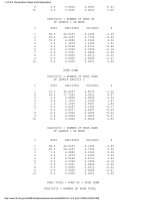
Analysis of
data
The level-1 standard deviation, which describes the basic precision of
the gauge, is
with v
1
= 2Q degrees of freedom.
The level-2 standard deviation, which describes the variability of the
measurement process over time, is
with v
2
= Q degrees of freedom.
Relationship
to
uncertainty
for a test
item
The standard deviation that defines the uncertainty for a single
measurement on a test item, often referred to as the reproducibility
standard deviation (ASTM), is given by
The time-dependent component is
There may be other sources of uncertainty in the measurement process
that must be accounted for in a formal analysis of uncertainty.
2.4.3.1. Simple design
(2 of 2) [5/1/2006 10:12:36 AM]