2. Measurement Process Characterization
2.3. Calibration
2.3.3. Calibration designs
2.3.3.2. General solutions to calibration designs
2.3.3.2.1.General matrix solutions to calibration
designs
Requirements Solutions for all designs that are cataloged in this Handbook are included with the designs.
Solutions for other designs can be computed from the instructions below given some
familiarity with matrices. The matrix manipulations that are required for the calculations are:
transposition (indicated by ')
●
multiplication●
inversion●
Notation n = number of difference measurements●
m = number of artifacts●
(n - m + 1) = degrees of freedom●
X= (nxm) design matrix●
r'= (mx1) vector identifying the restraint●
= (mx1) vector identifying ith item of interest consisting of a 1 in the ith position and
zeros elsewhere
●
R*= value of the reference standard●
Y= (mx1) vector of observed difference measurements●
Convention
for showing
the
measurement
sequence
The convention for showing the measurement sequence is illustrated with the three
measurements that make up a 1,1,1 design for 1 reference standard, 1 check standard, and 1
test item. Nominal values are underlined in the first line .

1 1 1
Y(1) = + -
Y(2) = + -
Y(3) = + -
2.3.3.2.1. General matrix solutions to calibration designs
(1 of 5) [5/1/2006 10:11:41 AM]
Matrix
algebra for
solving a
design
The (mxn) design matrix
X is constructed by replacing the pluses (+), minues (-) and blanks
with the entries 1, -1, and 0 respectively.
The (mxm) matrix of normal equations,
X'X, is formed and augmented by the restraint vector
to form an (m+1)x(m+1) matrix,
A:
Inverse of
design matrix
The
A matrix is inverted and shown in the form:
where Q is an mxm matrix that, when multiplied by s
2
, yields the usual variance-covariance
matrix.
Estimates of
values of
individual
artifacts
The least-squares estimates for the values of the individual artifacts are contained in the (mx1)

matrix,
B, where
where Q is the upper left element of the A
-1
matrix shown above. The structure of the
individual estimates is contained in the
QX' matrix; i.e. the estimate for the ith item can be
computed from
XQ and Y by
Cross multiplying the ith column of
XQ with Y●
And adding R*(nominal test)/(nominal restraint)●
Clarify with
an example
We will clarify the above discussion with an example from the mass calibration process at
NIST. In this example, two NIST kilograms are compared with a customer's unknown
kilogram.
The design matrix, X, is
The first two columns represent the two NIST kilograms while the third column represents the
customers kilogram (i.e., the kilogram being calibrated).
The measurements obtained, i.e., the Y matrix, are
2.3.3.2.1. General matrix solutions to calibration designs
(2 of 5) [5/1/2006 10:11:41 AM]
The measurements are the differences between two measurements, as specified by the design
matrix, measured in grams. That is, Y(1) is the difference in measurement between NIST
kilogram one and NIST kilogram two, Y(2) is the difference in measurement between NIST
kilogram one and the customer kilogram, and Y(3) is the difference in measurement between
NIST kilogram two and the customer kilogram.
The value of the reference standard,
R

*
, is 0.82329.
Then
If there are three weights with known values for weights one and two, then
r = [ 1 1 0 ]
Thus
and so
From A
-1
, we have
We then compute QX'
We then compute B = QX'Y + h'R
*
This yields the following least-squares coefficient estimates:
2.3.3.2.1. General matrix solutions to calibration designs
(3 of 5) [5/1/2006 10:11:41 AM]
Standard
deviations of
estimates
The standard deviation for the
ith item is:
where
The process standard deviation, which is a measure of the overall precision of the (NIST) mass
calibrarion process,
is the residual standard deviation from the design, and s
days
is the standard deviation for days,
which can only be estimated from check standard measurements.
Example We continue the example started above. Since n = 3 and m = 3, the formula reduces to:
Substituting the values shown above for X, Y, and Q results in

and
Y'(I - XQX')Y = 0.0000083333
Finally, taking the square root gives
s
1
= 0.002887
The next step is to compute the standard deviation of item 3 (the customers kilogram), that is
s
item
3
. We start by substitituting the values for X and Q and computing D
Next, we substitute = [0 0 1] and = 0.02111
2
(this value is taken from a check
standard and not computed from the values given in this example).
2.3.3.2.1. General matrix solutions to calibration designs
(4 of 5) [5/1/2006 10:11:41 AM]
We obtain the following computations
and
and
2.3.3.2.1. General matrix solutions to calibration designs
(5 of 5) [5/1/2006 10:11:41 AM]
2. Measurement Process Characterization
2.3. Calibration
2.3.3. What are calibration designs?
2.3.3.3. Uncertainties of calibrated values
2.3.3.3.1.Type A evaluations for calibration
designs
Change over
time

Type A evaluations for calibration processes must take into account
changes in the measurement process that occur over time.
Historically,
uncertainties
considered
only
instrument
imprecision
Historically, computations of uncertainties for calibrated values have
treated the precision of the comparator instrument as the primary
source of random uncertainty in the result. However, as the precision
of instrumentation has improved, effects of other sources of variability
have begun to show themselves in measurement processes. This is not
universally true, but for many processes, instrument imprecision
(short-term variability) cannot explain all the variation in the process.
Effects of
environmental
changes
Effects of humidity, temperature, and other environmental conditions
which cannot be closely controlled or corrected must be considered.
These tend to exhibit themselves over time, say, as between-day
effects. The discussion of between-day (level-2) effects relating to
gauge studies carries over to the calibration setting, but the
computations are not as straightforward.
Assumptions
which are
specific to
this section
The computations in this section depend on specific assumptions:
Short-term effects associated with instrument response

come from a single distribution
●
vary randomly from measurement to measurement within
a design.
●
1.
Day-to-day effects
come from a single distribution
●
vary from artifact to artifact but remain constant for a
single calibration
●
vary from calibration to calibration●
2.
2.3.3.3.1. Type A evaluations for calibration designs
(1 of 3) [5/1/2006 10:11:42 AM]
These
assumptions
have proved
useful but
may need to
be expanded
in the future
These assumptions have proved useful for characterizing high
precision measurement processes, but more complicated models may
eventually be needed which take the relative magnitudes of the test
items into account. For example, in mass calibration, a 100 g weight
can be compared with a summation of 50g, 30g and 20 g weights in a
single measurement. A sophisticated model might consider the size of
the effect as relative to the nominal masses or volumes.

Example of
the two
models for a
design for
calibrating
test item
using 1
reference
standard
To contrast the simple model with the more complicated model, a
measurement of the difference between X, the test item, with unknown
and yet to be determined value, X*, and a reference standard, R, with
known value, R*, and the reverse measurement are shown below.
Model (1) takes into account only instrument imprecision so that:
(1)
with the error terms random errors that come from the imprecision of
the measuring instrument.
Model (2) allows for both instrument imprecision and level-2 effects
such that:
(2)
where the delta terms explain small changes in the values of the
artifacts that occur over time. For both models, the value of the test
item is estimated as
2.3.3.3.1. Type A evaluations for calibration designs
(2 of 3) [5/1/2006 10:11:42 AM]
Standard
deviations
from both
models
For model (l), the standard deviation of the test item is

For model (2), the standard deviation of the test item is
.
Note on
relative
contributions
of both
components
to uncertainty
In both cases,
is the repeatability standard deviation that describes
the precision of the instrument and
is the level-2 standard
deviation that describes day-to-day changes. One thing to notice in the
standard deviation for the test item is the contribution of
relative to
the total uncertainty. If
is large relative to , or dominates, the
uncertainty will not be appreciably reduced by adding measurements
to the calibration design.
2.3.3.3.1. Type A evaluations for calibration designs
(3 of 3) [5/1/2006 10:11:42 AM]
Level-2
standard
deviation is
estimated
from check
standard
measurements
The level-2 standard deviation cannot be estimated from the data of the
calibration design. It cannot generally be estimated from repeated

designs involving the test items. The best mechanism for capturing the
day-to-day effects is a check standard, which is treated as a test item
and included in each calibration design. Values of the check standard,
estimated over time from the calibration design, are used to estimate
the standard deviation.
Assumptions The check standard value must be stable over time, and the
measurements must be in statistical control for this procedure to be
valid. For this purpose, it is necessary to keep a historical record of
values for a given check standard, and these values should be kept by
instrument and by design.
Computation
of level-2
standard
deviation
Given K historical check standard values,
the standard deviation of the check standard values is computed as
where
with degrees of freedom v = K - 1.
2.3.3.3.2. Repeatability and level-2 standard deviations
(2 of 2) [5/1/2006 10:11:43 AM]
2. Measurement Process Characterization
2.3. Calibration
2.3.3. What are calibration designs?
2.3.3.3. Uncertainties of calibrated values
2.3.3.3.4.Calculation of standard deviations for
1,1,1,1 design
Design with
2 reference
standards
and 2 test

items
An example is shown below for a 1,1,1,1 design for two reference standards, R
1
and R
2
,
and two test items, X
1
and X
2
, and six difference measurements. The restraint, R*, is the
sum of values of the two reference standards, and the check standard, which is
independent of the restraint, is the difference between the values of the reference
standards. The design and its solution are reproduced below.
Check
standard is
the
difference
between the
2 reference
standards
OBSERVATIONS 1 1 1 1
Y(1) + -
Y(2) + -
Y(3) + -
Y(4) + -
Y(5) + -
Y(6) + -
RESTRAINT + +


CHECK STANDARD + -


DEGREES OF FREEDOM = 3
SOLUTION MATRIX
2.3.3.3.4. Calculation of standard deviations for 1,1,1,1 design
(1 of 3) [5/1/2006 10:11:43 AM]
DIVISOR = 8
OBSERVATIONS 1 1 1 1
Y(1) 2 -2 0 0
Y(2) 1 -1 -3 -1
Y(3) 1 -1 -1 -3
Y(4) -1 1 -3 -1
Y(5) -1 1 -1 -3
Y(6) 0 0 2 -2
R* 4 4 4 4
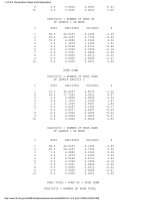
Explanation
of solution
matrix
The solution matrix gives values for the test items of
Factors for
computing
contributions
of
repeatability
and level-2
standard
deviations to
uncertainty
FACTORS FOR REPEATABILITY STANDARD

DEVIATIONS
WT FACTOR
K
1
1 1 1 1
1 0.3536 +
1 0.3536 +
1 0.6124 +
1 0.6124 +
0 0.7071 + -

FACTORS FOR LEVEL-2 STANDARD DEVIATIONS
WT FACTOR
K
2
1 1 1 1
1 0.7071 +
1 0.7071 +
1 1.2247 +
2.3.3.3.4. Calculation of standard deviations for 1,1,1,1 design
(2 of 3) [5/1/2006 10:11:43 AM]
1 1.2247 +
0 1.4141 + -
The first table shows factors for computing the contribution of the repeatability
standard deviation to the total uncertainty. The second table shows factors for
computing the contribution of the between-day standard deviation to the uncertainty.
Notice that the check standard is the last entry in each table.
Unifying
equation
The unifying equation is:

Standard
deviations
are
computed
using the
factors from
the tables
with the
unifying
equation
The steps in computing the standard deviation for a test item are:
Compute the repeatability standard deviation from historical data.●
Compute the standard deviation of the check standard from historical data.●
Locate the factors, K
1
and K
2
, for the check standard.●
Compute the between-day variance (using the unifying equation for the check
standard). For this example,
.
●
If this variance estimate is negative, set = 0. (This is possible and
indicates that there is no contribution to uncertainty from day-to-day effects.)
●
Locate the factors, K
1
and K
2
, for the test items, and compute the standard

deviations using the unifying equation. For this example,
and
●
2.3.3.3.4. Calculation of standard deviations for 1,1,1,1 design
(3 of 3) [5/1/2006 10:11:43 AM]
2.3.3.3.5. Type B uncertainty
(2 of 2) [5/1/2006 10:11:44 AM]
Degrees of freedom
using the
Welch-Satterthwaite
approximation
Therefore, the degrees of freedom is approximated as
where n - 1 is the degrees of freedom associated with the check standard uncertainty.
Notice that the standard deviation of the restraint drops out of the calculation because
of an infinite degrees of freedom.
2.3.3.3.6. Expanded uncertainties
(2 of 2) [5/1/2006 10:11:44 AM]
Information:
Design
Solution
Factors for
computing
standard
deviations
Given
n = number of difference measurements
●
m = number of artifacts (reference standards + test items) to be calibrated●
the following information is shown for each design:
Design matrix (n x m)

●
Vector that identifies standards in the restraint (1 x m)●
Degrees of freedom = (n - m + 1)●
Solution matrix for given restraint (n x m)●
Table of factors for computing standard deviations●
Convention
for showing
the
measurement
sequence
Nominal sizes of standards and test items are shown at the top of the design. Pluses (+)
indicate items that are measured together; and minuses (-) indicate items are not
measured together. The difference measurements are constructed from the design of
pluses and minuses. For example, a 1,1,1 design for one reference standard and two test
items of the same nominal size with three measurements is shown below:
1 1 1
Y(1) = + -
Y(2) = + -
Y(3) = + -

Solution
matrix
Example and
interpretation
The cross-product of the column of difference measurements and R* with a column
from the solution matrix, divided by the named divisor, gives the value for an individual
item. For example,
Solution matrix
Divisor = 3


1 1 1
Y(1) 0 -2 -1
Y(2) 0 -1 -2
Y(3) 0 +1 -1
R* +3 +3 +3
implies that estimates for the restraint and the two test items are:
2.3.4. Catalog of calibration designs
(2 of 3) [5/1/2006 10:11:45 AM]
Interpretation
of table of
factors
The factors in this table provide information on precision. The repeatability standard
deviation,
, is multiplied by the appropriate factor to obtain the standard deviation for
an individual item or combination of items. For example,

Sum Factor 1 1 1
1 0.0000 +
1 0.8166 +
1 0.8166 +
2 1.4142 + +
implies that the standard deviations for the estimates are:
2.3.4. Catalog of calibration designs
(3 of 3) [5/1/2006 10:11:45 AM]
First series
using
1,1,1,1
design
The calibrations start with a comparison of the one kilogram test weight
with the reference kilograms (see the graphic above). The 1,1,1,1 design

requires two kilogram reference standards with known values, R1* and
R2*. The fourth kilogram in this design is actually a summation of the
500, 300, 200 g weights which becomes the restraint in the next series.
The restraint for the first series is the known average mass of the
reference kilograms,
The design assigns values to all weights including the individual
reference standards. For this design, the check standard is not an artifact
standard but is defined as the difference between the values assigned to
the reference kilograms by the design; namely,
2.3.4.1. Mass weights
(2 of 4) [5/1/2006 10:11:45 AM]
2nd series
using
5,3,2,1,1,1
design
The second series is a 5,3,2,1,1,1 design where the restraint over the
500g, 300g and 200g weights comes from the value assigned to the
summation in the first series; i.e.,
The weights assigned values by this series are:
500g, 300g, 200 g and 100g test weights
●
100 g check standard (2nd 100g weight in the design)●
Summation of the 50g, 30g, 20g weights.●
Other
starting
points
The calibration sequence can also start with a 1,1,1 design. This design
has the disadvantage that it does not have provision for a check
standard.
Better

choice of
design
A better choice is a 1,1,1,1,1 design which allows for two reference
kilograms and a kilogram check standard which occupies the 4th
position among the weights. This is preferable to the 1,1,1,1 design but
has the disadvantage of requiring the laboratory to maintain three
kilogram standards.
Important
detail
The solutions are only applicable for the restraints as shown.
Designs for
decreasing
weight sets
1,1,1 design1.
1,1,1,1 design2.
1,1,1,1,1 design3.
1,1,1,1,1,1 design4.
2,1,1,1 design5.
2,2,1,1,1 design6.
2,2,2,1,1 design7.
5,2,2,1,1,1 design8.
5,2,2,1,1,1,1 design9.
5,3,2,1,1,1 design10.
5,3,2,1,1,1,1 design11.
5,3,2,2,1,1,1 design12.
5,4,4,3,2,2,1,1 design13.
5,5,2,2,1,1,1,1 design14.
2.3.4.1. Mass weights
(3 of 4) [5/1/2006 10:11:45 AM]