9 0.0 0.0000 0.0065 -0.01
10 0.0 0.0000 0.0020 0.00


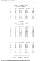
STATISTIC = NUMBER OF RUNS UP
OF LENGTH I OR MORE

I STAT EXP(STAT) SD(STAT) Z

1 58.0 64.8333 4.1439 -1.65
2 23.0 24.1667 2.7729 -0.42
3 15.0 6.4083 2.1363 4.02
4 3.0 1.3278 1.1043 1.51
5 0.0 0.2264 0.4716 -0.48
6 0.0 0.0328 0.1809 -0.18
7 0.0 0.0041 0.0644 -0.06
8 0.0 0.0005 0.0215 -0.02
9 0.0 0.0000 0.0068 -0.01
10 0.0 0.0000 0.0021 0.00


RUNS DOWN

STATISTIC = NUMBER OF RUNS DOWN
OF LENGTH EXACTLY I

I STAT EXP(STAT) SD(STAT) Z

1 33.0 40.6667 6.4079 -1.20
2 18.0 17.7583 3.3021 0.07
3 3.0 5.0806 2.0096 -1.04

4 3.0 1.1014 1.0154 1.87
5 1.0 0.1936 0.4367 1.85
6 0.0 0.0287 0.1692 -0.17
7 0.0 0.0037 0.0607 -0.06
8 0.0 0.0004 0.0204 -0.02
9 0.0 0.0000 0.0065 -0.01
10 0.0 0.0000 0.0020 0.00


STATISTIC = NUMBER OF RUNS DOWN
OF LENGTH I OR MORE


I STAT EXP(STAT) SD(STAT) Z

1 58.0 64.8333 4.1439 -1.65
2 25.0 24.1667 2.7729 0.30
3 7.0 6.4083 2.1363 0.28
4 4.0 1.3278 1.1043 2.42
5 1.0 0.2264 0.4716 1.64
6 0.0 0.0328 0.1809 -0.18
7 0.0 0.0041 0.0644 -0.06
8 0.0 0.0005 0.0215 -0.02
9 0.0 0.0000 0.0068 -0.01
10 0.0 0.0000 0.0021 0.00


RUNS TOTAL = RUNS UP + RUNS DOWN

STATISTIC = NUMBER OF RUNS TOTAL

1.4.2.8.3. Quantitative Output and Interpretation
(4 of 8) [5/1/2006 9:58:59 AM]
OF LENGTH EXACTLY I

I STAT EXP(STAT) SD(STAT) Z

1 68.0 81.3333 9.0621 -1.47
2 26.0 35.5167 4.6698 -2.04
3 15.0 10.1611 2.8420 1.70
4 6.0 2.2028 1.4360 2.64
5 1.0 0.3871 0.6176 0.99
6 0.0 0.0574 0.2392 -0.24
7 0.0 0.0074 0.0858 -0.09
8 0.0 0.0008 0.0289 -0.03
9 0.0 0.0001 0.0092 -0.01
10 0.0 0.0000 0.0028 0.00


STATISTIC = NUMBER OF RUNS TOTAL
OF LENGTH I OR MORE

I STAT EXP(STAT) SD(STAT) Z

1 116.0 129.6667 5.8604 -2.33
2 48.0 48.3333 3.9215 -0.09
3 22.0 12.8167 3.0213 3.04
4 7.0 2.6556 1.5617 2.78
5 1.0 0.4528 0.6669 0.82
6 0.0 0.0657 0.2559 -0.26
7 0.0 0.0083 0.0911 -0.09

8 0.0 0.0009 0.0305 -0.03
9 0.0 0.0001 0.0097 -0.01
10 0.0 0.0000 0.0029 0.00


LENGTH OF THE LONGEST RUN UP = 4
LENGTH OF THE LONGEST RUN DOWN = 5
LENGTH OF THE LONGEST RUN UP OR DOWN = 5

NUMBER OF POSITIVE DIFFERENCES = 98
NUMBER OF NEGATIVE DIFFERENCES = 95
NUMBER OF ZERO DIFFERENCES = 1

Values in the column labeled "Z" greater than 1.96 or less than -1.96 are statistically
significant at the 5% level. The runs test does indicate some non-randomness.
Although the autocorrelation plot and the runs test indicate some mild non-randomness,
the violation of the randomness assumption is not serious enough to warrant developing a
more sophisticated model. It is common in practice that some of the assumptions are
mildly violated and it is a judgement call as to whether or not the violations are serious
enough to warrant developing a more sophisticated model for the data.
1.4.2.8.3. Quantitative Output and Interpretation
(5 of 8) [5/1/2006 9:58:59 AM]
Distributional
Analysis
Probability plots are a graphical test for assessing if a particular distribution provides an
adequate fit to a data set.
A quantitative enhancement to the probability plot is the correlation coefficient of the
points on the probability plot. For this data set the correlation coefficient is 0.996. Since
this is greater than the critical value of 0.987 (this is a tabulated value), the normality
assumption is not rejected.

Chi-square and Kolmogorov-Smirnov goodness-of-fit tests are alternative methods for
assessing distributional adequacy. The Wilk-Shapiro and Anderson-Darling tests can be
used to test for normality. Dataplot generates the following output for the
Anderson-Darling normality test.

ANDERSON-DARLING 1-SAMPLE TEST
THAT THE DATA CAME FROM A NORMAL DISTRIBUTION

1. STATISTICS:
NUMBER OF OBSERVATIONS = 195
MEAN = 9.261460
STANDARD DEVIATION = 0.2278881E-01

ANDERSON-DARLING TEST STATISTIC VALUE = 0.1264954
ADJUSTED TEST STATISTIC VALUE = 0.1290070

2. CRITICAL VALUES:
90 % POINT = 0.6560000
95 % POINT = 0.7870000
97.5 % POINT = 0.9180000
99 % POINT = 1.092000

3. CONCLUSION (AT THE 5% LEVEL):
THE DATA DO COME FROM A NORMAL DISTRIBUTION.

The Anderson-Darling test also does not reject the normality assumption because the test
statistic, 0.129, is less than the critical value at the 5% significance level of 0.918.
Outlier
Analysis
A test for outliers is the Grubbs' test. Dataplot generated the following output for Grubbs'

test.

GRUBBS TEST FOR OUTLIERS
(ASSUMPTION: NORMALITY)

1. STATISTICS:
NUMBER OF OBSERVATIONS = 195
MINIMUM = 9.196848
MEAN = 9.261460
MAXIMUM = 9.327973
STANDARD DEVIATION = 0.2278881E-01

GRUBBS TEST STATISTIC = 2.918673

2. PERCENT POINTS OF THE REFERENCE DISTRIBUTION
1.4.2.8.3. Quantitative Output and Interpretation
(6 of 8) [5/1/2006 9:58:59 AM]
FOR GRUBBS TEST STATISTIC
0 % POINT = 0.000000
50 % POINT = 2.984294
75 % POINT = 3.181226
90 % POINT = 3.424672
95 % POINT = 3.597898
97.5 % POINT = 3.763061
99 % POINT = 3.970215
100 % POINT = 13.89263

3. CONCLUSION (AT THE 5% LEVEL):
THERE ARE NO OUTLIERS.


For this data set, Grubbs' test does not detect any outliers at the 25%, 10%, 5%, and 1%
significance levels.
Model Since the underlying assumptions were validated both graphically and analytically, with a
mild violation of the randomness assumption, we conclude that a reasonable model for
the data is:
We can express the uncertainty for C, here estimated by 9.26146, as the 95% confidence
interval (9.258242,9.26479).
Univariate
Report
It is sometimes useful and convenient to summarize the above results in a report. The
report for the heat flow meter data follows.

Analysis for heat flow meter data

1: Sample Size = 195

2: Location
Mean = 9.26146
Standard Deviation of Mean = 0.001632
95% Confidence Interval for Mean = (9.258242,9.264679)
Drift with respect to location? = NO

3: Variation
Standard Deviation = 0.022789
95% Confidence Interval for SD = (0.02073,0.025307)
Drift with respect to variation?
(based on Bartlett's test on quarters
of the data) = NO

4: Randomness

Autocorrelation = 0.280579
Data are Random?
(as measured by autocorrelation) = NO

5: Distribution
Normal PPCC = 0.998965
Data are Normal?
(as measured by Normal PPCC) = YES

6: Statistical Control
(i.e., no drift in location or scale,
1.4.2.8.3. Quantitative Output and Interpretation
(7 of 8) [5/1/2006 9:58:59 AM]
data are random, distribution is
fixed, here we are testing only for
fixed normal)
Data Set is in Statistical Control? = YES

7: Outliers?
(as determined by Grubbs' test) = NO

1.4.2.8.3. Quantitative Output and Interpretation
(8 of 8) [5/1/2006 9:58:59 AM]
4. Generate a normal probability
plot.
4. The normal probability plot verifies
that the normal distribution is a
reasonable distribution for these data.
4. Generate summary statistics, quantitative
analysis, and print a univariate report.

1. Generate a table of summary
statistics.
2. Generate the mean, a confidence
interval for the mean, and compute
a linear fit to detect drift in
location.
3. Generate the standard deviation, a
confidence interval for the standard
deviation, and detect drift in variation
by dividing the data into quarters and
computing Bartlett's test for equal
standard deviations.
4. Check for randomness by generating an
autocorrelation plot and a runs test.
5. Check for normality by computing the
normal probability plot correlation
coefficient.
6. Check for outliers using Grubbs' test.
7. Print a univariate report (this assumes
steps 2 thru 6 have already been run).
1. The summary statistics table displays
25+ statistics.
2. The mean is 9.261 and a 95%
confidence interval is (9.258,9.265).
The linear fit indicates no drift in
location since the slope parameter
estimate is essentially zero.
3. The standard deviation is 0.023 with
a 95% confidence interval of (0.0207,0.0253).
Bartlett's test indicates no significant

change in variation.
4. The lag 1 autocorrelation is 0.28.
From the autocorrelation plot, this is
statistically significant at the 95%
level.
5. The normal probability plot correlation
coefficient is 0.999. At the 5% level,
we cannot reject the normality assumption.
6. Grubbs' test detects no outliers at the
5% level.
7. The results are summarized in a
convenient report.
1.4.2.8.4. Work This Example Yourself
(2 of 2) [5/1/2006 9:58:59 AM]
1. Exploratory Data Analysis
1.4. EDA Case Studies
1.4.2. Case Studies
1.4.2.9. Airplane Polished Window Strength
1.4.2.9.1.Background and Data
Generation This data set was provided by Ed Fuller of the NIST Ceramics Division
in December, 1993. It contains polished window strength data that was
used with two other sets of data (constant stress-rate data and strength of
indented glass data). A paper by Fuller, et. al. describes the use of all
three data sets to predict lifetime and confidence intervals for a glass
airplane window. A paper by Pepi describes the all-glass airplane
window design.
For this case study, we restrict ourselves to the problem of finding a
good distributional model of the polished window strength data.
Purpose of
Analysis

The goal of this case study is to find a good distributional model for the
polished window strength data. Once a good distributional model has
been determined, various percent points for the polished widow strength
will be computed.
Since the data were used in a study to predict failure times, this case
study is a form of reliability analysis. The assessing product reliability
chapter contains a more complete discussion of reliabilty methods. This
case study is meant to complement that chapter by showing the use of
graphical techniques in one aspect of reliability modeling.
Data in reliability analysis do not typically follow a normal distribution;
non-parametric methods (techniques that do not rely on a specific
distribution) are frequently recommended for developing confidence
intervals for failure data. One problem with this approach is that sample
sizes are often small due to the expense involved in collecting the data,
and non-parametric methods do not work well for small sample sizes.
For this reason, a parametric method based on a specific distributional
model of the data is preferred if the data can be shown to follow a
specific distribution. Parametric models typically have greater efficiency
at the cost of more specific assumptions about the data, but, it is
important to verify that the distributional assumption is indeed valid. If
the distributional assumption is not justified, then the conclusions drawn
1.4.2.9.1. Background and Data
(1 of 2) [5/1/2006 9:58:59 AM]
from the model may not be valid.
This file can be read by Dataplot with the following commands:
SKIP 25
READ FULLER2.DAT Y
Resulting
Data
The following are the data used for this case study. The data are in ksi

(= 1,000 psi).
18.830
20.800
21.657
23.030
23.230
24.050
24.321
25.500
25.520
25.800
26.690
26.770
26.780
27.050
27.670
29.900
31.110
33.200
33.730
33.760
33.890
34.760
35.750
35.910
36.980
37.080
37.090
39.580
44.045

45.290
45.381
1.4.2.9.1. Background and Data
(2 of 2) [5/1/2006 9:58:59 AM]
The normal probability plot has a correlation coefficient of 0.980. We can use
this number as a reference baseline when comparing the performance of other
distributional fits.
Other Potential
Distributions
There is a large number of distributions that would be distributional model
candidates for the data. However, we will restrict ourselves to consideration of
the following distributional models because these have proven to be useful in
reliability studies.
Normal distribution1.
Exponential distribution2.
Weibull distribution3.
Lognormal distribution4.
Gamma distribution5.
Power normal distribution6.
Fatigue life distribution7.
1.4.2.9.2. Graphical Output and Interpretation
(2 of 7) [5/1/2006 9:59:00 AM]
Approach There are two basic questions that need to be addressed.
Does a given distributional model provide an adequate fit to the data?1.
Of the candidate distributional models, is there one distribution that fits
the data better than the other candidate distributional models?
2.
The use of probability plots and probability plot correlation coefficient (PPCC)
plots provide answers to both of these questions.
If the distribution does not have a shape parameter, we simply generate a

probability plot.
If we fit a straight line to the points on the probability plot, the intercept
and slope of that line provide estimates of the location and scale
parameters, respectively.
1.
Our critierion for the "best fit" distribution is the one with the most linear
probability plot. The correlation coefficient of the fitted line of the points
on the probability plot, referred to as the PPCC value, provides a measure
of the linearity of the probability plot, and thus a measure of how well the
distribution fits the data. The PPCC values for multiple distributions can
be compared to address the second question above.
2.
If the distribution does have a shape parameter, then we are actually addressing
a family of distributions rather than a single distribution. We first need to find
the optimal value of the shape parameter. The PPCC plot can be used to
determine the optimal parameter. We will use the PPCC plots in two stages. The
first stage will be over a broad range of parameter values while the second stage
will be in the neighborhood of the largest values. Although we could go further
than two stages, for practical purposes two stages is sufficient. After
determining an optimal value for the shape parameter, we use the probability
plot as above to obtain estimates of the location and scale parameters and to
determine the PPCC value. This PPCC value can be compared to the PPCC
values obtained from other distributional models.
Analyses for
Specific
Distributions
We analyzed the data using the approach described above for the following
distributional models:
Normal distribution - from the 4-plot above, the PPCC value was 0.980.1.
Exponential distribution - the exponential distribution is a special case of

the Weibull with shape parameter equal to 1. If the Weibull analysis
yields a shape parameter close to 1, then we would consider using the
simpler exponential model.
2.
Weibull distribution3.
Lognormal distribution4.
Gamma distribution5.
Power normal distribution6.
Power lognormal distribution7.
1.4.2.9.2. Graphical Output and Interpretation
(3 of 7) [5/1/2006 9:59:00 AM]
Summary of
Results
The results are summarized below.
Normal Distribution
Max PPCC = 0.980
Estimate of location = 30.81
Estimate of scale = 7.38
Weibull Distribution
Max PPCC = 0.988
Estimate of shape = 2.13
Estimate of location = 15.9
Estimate of scale = 16.92
Lognormal Distribution
Max PPCC = 0.986
Estimate of shape = 0.18
Estimate of location = -9.96
Estimate of scale = 40.17
Gamma Distribution
Max PPCC = 0.987

Estimate of shape = 11.8
Estimate of location = 5.19
Estimate of scale = 2.17
Power Normal Distribution
Max PPCC = 0.988
Estimate of shape = 0.05
Estimate of location = 19.0
Estimate of scale = 2.4
Fatigue Life Distribution
Max PPCC = 0.987
Estimate of shape = 0.18
Estimate of location = -11.0
Estimate of scale = 41.3
These results indicate that several of these distributions provide an adequate
distributional model for the data. We choose the 3-parameter Weibull
distribution as the most appropriate model because it provides the best balance
between simplicity and best fit.
1.4.2.9.2. Graphical Output and Interpretation
(4 of 7) [5/1/2006 9:59:00 AM]
Percent Point
Estimates
The final step in this analysis is to compute percent point estimates for the 1%,
2.5%, 5%, 95%, 97.5%, and 99% percent points. A percent point estimate is an
estimate of the strength at which a given percentage of units will be weaker. For
example, the 5% point is the strength at which we estimate that 5% of the units
will be weaker.
To calculate these values, we use the Weibull percent point function with the
appropriate estimates of the shape, location, and scale parameters. The Weibull
percent point function can be computed in many general purpose statistical
software programs, including Dataplot.

Dataplot generated the following estimates for the percent points:
Estimated percent points using Weibull Distribution

PERCENT POINT POLISHED WINDOW STRENGTH
0.01 17.86
0.02 18.92
0.05 20.10
0.95 44.21
0.97 47.11
0.99 50.53
Quantitative
Measures of
Goodness of Fit
Although it is generally unnecessary, we can include quantitative measures of
distributional goodness-of-fit. Three of the commonly used measures are:
Chi-square goodness-of-fit.1.
Kolmogorov-Smirnov goodness-of-fit.2.
Anderson-Darling goodness-of-fit.3.
In this case, the sample size of 31 precludes the use of the chi-square test since
the chi-square approximation is not valid for small sample sizes. Specifically,
the smallest expected frequency should be at least 5. Although we could
combine classes, we will instead use one of the other tests. The
Kolmogorov-Smirnov test requires a fully specified distribution. Since we need
to use the data to estimate the shape, location, and scale parameters, we do not
use this test here. The Anderson-Darling test is a refinement of the
Kolmogorov-Smirnov test. We run this test for the normal, lognormal, and
Weibull distributions.
1.4.2.9.2. Graphical Output and Interpretation
(5 of 7) [5/1/2006 9:59:00 AM]
Normal

Anderson-Darling
Output
ANDERSON-DARLING 1-SAMPLE TEST
THAT THE DATA CAME FROM A NORMAL DISTRIBUTION

1. STATISTICS:
NUMBER OF OBSERVATIONS = 31
MEAN = 30.81142
STANDARD DEVIATION = 7.253381

ANDERSON-DARLING TEST STATISTIC VALUE = 0.5321903
ADJUSTED TEST STATISTIC VALUE = 0.5870153

2. CRITICAL VALUES:
90 % POINT = 0.6160000
95 % POINT = 0.7350000
97.5 % POINT = 0.8610000
99 % POINT = 1.021000

3. CONCLUSION (AT THE 5% LEVEL):
THE DATA DO COME FROM A NORMAL DISTRIBUTION.
Lognormal
Anderson-Darling
Output
ANDERSON-DARLING 1-SAMPLE TEST
THAT THE DATA CAME FROM A LOGNORMAL DISTRIBUTION

1. STATISTICS:
NUMBER OF OBSERVATIONS = 31
MEAN OF LOG OF DATA = 3.401242

STANDARD DEVIATION OF LOG OF DATA = 0.2349026

ANDERSON-DARLING TEST STATISTIC VALUE = 0.3888340
ADJUSTED TEST STATISTIC VALUE = 0.4288908

2. CRITICAL VALUES:
90 % POINT = 0.6160000
95 % POINT = 0.7350000
97.5 % POINT = 0.8610000
99 % POINT = 1.021000

3. CONCLUSION (AT THE 5% LEVEL):
THE DATA DO COME FROM A LOGNORMAL DISTRIBUTION.
1.4.2.9.2. Graphical Output and Interpretation
(6 of 7) [5/1/2006 9:59:00 AM]
Weibull
Anderson-Darling
Output
ANDERSON-DARLING 1-SAMPLE TEST
THAT THE DATA CAME FROM A WEIBULL DISTRIBUTION

1. STATISTICS:
NUMBER OF OBSERVATIONS = 31
MEAN = 14.91142
STANDARD DEVIATION = 7.253381
SHAPE PARAMETER = 2.237495
SCALE PARAMETER = 16.87868

ANDERSON-DARLING TEST STATISTIC VALUE = 0.3623638
ADJUSTED TEST STATISTIC VALUE = 0.3753803


2. CRITICAL VALUES:
90 % POINT = 0.6370000
95 % POINT = 0.7570000
97.5 % POINT = 0.8770000
99 % POINT = 1.038000

3. CONCLUSION (AT THE 5% LEVEL):
THE DATA DO COME FROM A WEIBULL DISTRIBUTION.
Note that for the Weibull distribution, the Anderson-Darling test is actually
testing the 2-parameter Weibull distribution (based on maximum likelihood
estimates), not the 3-parameter Weibull distribution. To give a more accurate
comparison, we subtract the location parameter (15.9) as estimated by the PPCC
plot/probability plot technique before applying the Anderson-Darling test.
Conclusions The Anderson-Darling test passes all three of these distributions. Note that the
value of the Anderson-Darling test statistic is the smallest for the Weibull
distribution with the value for the lognormal distribution just slightly larger. The
test statistic for the normal distribution is noticeably higher than for the Weibull
or lognormal.
This provides additional confirmation that either the Weibull or lognormal
distribution fits this data better than the normal distribution with the Weibull
providing a slightly better fit than the lognormal.
1.4.2.9.2. Graphical Output and Interpretation
(7 of 7) [5/1/2006 9:59:00 AM]
Alternative
Plots
The Weibull plot and the Weibull hazard plot are alternative graphical
analysis procedures to the PPCC plots and probability plots.
These two procedures, especially the Weibull plot, are very commonly
employed. That not withstanding, the disadvantage of these two

procedures is that they both assume that the location parameter (i.e., the
lower bound) is zero and that we are fitting a 2-parameter Weibull
instead of a 3-parameter Weibull. The advantage is that there is an
extensive literature on these methods and they have been designed to
work with either censored or uncensored data.
Weibull Plot
This Weibull plot shows the following
The Weibull plot is approximately linear indicating that the
2-parameter Weibull provides an adequate fit to the data.
1.
The estimate of the shape parameter is 5.28 and the estimate of
the scale parameter is 33.32.
2.
1.4.2.9.3. Weibull Analysis
(2 of 3) [5/1/2006 9:59:00 AM]
Weibull
Hazard Plot
The construction and interpretation of the Weibull hazard plot is
discussed in the Assessing Product Reliability chapter.
1.4.2.9.3. Weibull Analysis
(3 of 3) [5/1/2006 9:59:00 AM]
1.4.2.9.4. Lognormal Analysis
(2 of 2) [5/1/2006 9:59:01 AM]
1.4.2.9.5. Gamma Analysis
(2 of 2) [5/1/2006 9:59:01 AM]