the outlying point).
1.3.3.26.10. Scatter Plot: Outlier
(2 of 2) [5/1/2006 9:57:06 AM]
1. Exploratory Data Analysis
1.3. EDA Techniques
1.3.3. Graphical Techniques: Alphabetic
1.3.3.26. Scatter Plot
1.3.3.26.11.Scatterplot Matrix
Purpose:
Check
Pairwise
Relationships
Between
Variables
Given a set of variables X
1
, X
2
, , X
k
, the scatterplot matrix contains
all the pairwise scatter plots of the variables on a single page in a
matrix format. That is, if there are k variables, the scatterplot matrix
will have k rows and k columns and the ith row and jth column of this
matrix is a plot of X
i
versus X
j
.
Although the basic concept of the scatterplot matrix is simple, there are
numerous alternatives in the details of the plots.

The diagonal plot is simply a 45-degree line since we are plotting
X
i
versus X
i
. Although this has some usefulness in terms of
showing the univariate distribution of the variable, other
alternatives are common. Some users prefer to use the diagonal
to print the variable label. Another alternative is to plot the
univariate histogram on the diagonal. Alternatively, we could
simply leave the diagonal blank.
1.
Since X
i
versus X
j
is equivalent to X
j
versus X
i
with the axes
reversed, some prefer to omit the plots below the diagonal.
2.
It can be helpful to overlay some type of fitted curve on the
scatter plot. Although a linear or quadratic fit can be used, the
most common alternative is to overlay a lowess curve.
3.
Due to the potentially large number of plots, it can be somewhat
tricky to provide the axes labels in a way that is both informative
and visually pleasing. One alternative that seems to work well is

to provide axis labels on alternating rows and columns. That is,
row one will have tic marks and axis labels on the left vertical
axis for the first plot only while row two will have the tic marks
and axis labels for the right vertical axis for the last plot in the
row only. This alternating pattern continues for the remaining
rows. A similar pattern is used for the columns and the horizontal
axes labels. Another alternative is to put the minimum and
maximum scale value in the diagonal plot with the variable
4.
1.3.3.26.11. Scatterplot Matrix
(1 of 3) [5/1/2006 9:57:06 AM]
name.
Some analysts prefer to connect the scatter plots. Others prefer to
leave a little gap between each plot.
5.
Although this plot type is most commonly used for scatter plots,
the basic concept is both simple and powerful and extends easily
to other plot formats that involve pairwise plots such as the
quantile-quantile plot and the bihistogram.
6.
Sample Plot
This sample plot was generated from pollution data collected by NIST
chemist Lloyd Currie.
There are a number of ways to view this plot. If we are primarily
interested in a particular variable, we can scan the row and column for
that variable. If we are interested in finding the strongest relationship,
we can scan all the plots and then determine which variables are
related.
Definition Given k variables, scatter plot matrices are formed by creating k rows
and k columns. Each row and column defines a single scatter plot

The individual plot for row i and column j is defined as
Vertical axis: Variable X
i
●
Horizontal axis: Variable X
j
●
1.3.3.26.11. Scatterplot Matrix
(2 of 3) [5/1/2006 9:57:06 AM]
Questions The scatterplot matrix can provide answers to the following questions:
Are there pairwise relationships between the variables?1.
If there are relationships, what is the nature of these
relationships?
2.
Are there outliers in the data?3.
Is there clustering by groups in the data?4.
Linking and
Brushing
The scatterplot matrix serves as the foundation for the concepts of
linking and brushing.
By linking, we mean showing how a point, or set of points, behaves in
each of the plots. This is accomplished by highlighting these points in
some fashion. For example, the highlighted points could be drawn as a
filled circle while the remaining points could be drawn as unfilled
circles. A typical application of this would be to show how an outlier
shows up in each of the individual pairwise plots. Brushing extends this
concept a bit further. In brushing, the points to be highlighted are
interactively selected by a mouse and the scatterplot matrix is
dynamically updated (ideally in real time). That is, we can select a
rectangular region of points in one plot and see how those points are

reflected in the other plots. Brushing is discussed in detail by Becker,
Cleveland, and Wilks in the paper "Dynamic Graphics for Data
Analysis" (Cleveland and McGill, 1988).
Related
Techniques
Star plot
Scatter plot
Conditioning plot
Locally weighted least squares
Software Scatterplot matrices are becoming increasingly common in general
purpose statistical software programs, including Dataplot. If a software
program does not generate scatterplot matrices, but it does provide
multiple plots per page and scatter plots, it should be possible to write a
macro to generate a scatterplot matrix. Brushing is available in a few of
the general purpose statistical software programs that emphasize
graphical approaches.
1.3.3.26.11. Scatterplot Matrix
(3 of 3) [5/1/2006 9:57:06 AM]
Although this plot type is most commonly used for scatter plots,
the basic concept is both simple and powerful and extends easily
to other plot formats.
4.
Sample Plot
In this case, temperature has six distinct values. We plot torque versus
time for each of these temperatures. This example is discussed in more
detail in the process modeling chapter.
Definition Given the variables X, Y, and Z, the conditioning plot is formed by
dividing the values of Z into k groups. There are several ways that these
groups may be formed. There may be a natural grouping of the data, the
data may be divided into several equal sized groups, the grouping may

be determined by clusters in the data, and so on. The page will be
divided into n rows and c columns where
. Each row and
column defines a single scatter plot.
The individual plot for row i and column j is defined as
Vertical axis: Variable Y●
Horizontal axis: Variable X●
where only the points in the group corresponding to the ith row and jth
column are used.
1.3.3.26.12. Conditioning Plot
(2 of 3) [5/1/2006 9:57:06 AM]
Questions The conditioning plot can provide answers to the following questions:
Is there a relationship between two variables?1.
If there is a relationship, does the nature of the relationship
depend on the value of a third variable?
2.
Are groups in the data similar?3.
Are there outliers in the data?4.
Related
Techniques
Scatter plot
Scatterplot matrix
Locally weighted least squares
Software Scatter plot matrices are becoming increasingly common in general
purpose statistical software programs, including Dataplot. If a software
program does not generate conditioning plots, but it does provide
multiple plots per page and scatter plots, it should be possible to write a
macro to generate a conditioning plot.
1.3.3.26.12. Conditioning Plot
(3 of 3) [5/1/2006 9:57:06 AM]

Sample Plot
This spectral plot shows one dominant frequency of approximately 0.3
cycles per observation.
Definition:
Variance
Versus
Frequency
The spectral plot is formed by:
Vertical axis: Smoothed variance (power)
●
Horizontal axis: Frequency (cycles per observation)●
The computations for generating the smoothed variances can be
involved and are not discussed further here. The details can be found in
the Jenkins and Bloomfield references and in most texts that discuss the
frequency analysis of time series.
Questions The spectral plot can be used to answer the following questions:
How many cyclic components are there?1.
Is there a dominant cyclic frequency?2.
If there is a dominant cyclic frequency, what is it?3.
Importance
Check
Cyclic
Behavior of
Time Series
The spectral plot is the primary technique for assessing the cyclic nature
of univariate time series in the frequency domain. It is almost always the
second plot (after a run sequence plot) generated in a frequency domain
analysis of a time series.
1.3.3.27. Spectral Plot
(2 of 3) [5/1/2006 9:57:07 AM]

Examples Random (= White Noise)1.
Strong autocorrelation and autoregressive model2.
Sinusoidal model3.
Related
Techniques
Autocorrelation Plot
Complex Demodulation Amplitude Plot
Complex Demodulation Phase Plot
Case Study
The spectral plot is demonstrated in the beam deflection data case study.
Software Spectral plots are a fundamental technique in the frequency analysis of
time series. They are available in many general purpose statistical
software programs, including Dataplot.
1.3.3.27. Spectral Plot
(3 of 3) [5/1/2006 9:57:07 AM]
1.3.3.27.1. Spectral Plot: Random Data
(2 of 2) [5/1/2006 9:57:07 AM]
Discussion This spectral plot starts with a dominant peak near zero and rapidly
decays to zero. This is the spectral plot signature of a process with
strong positive autocorrelation. Such processes are highly non-random
in that there is high association between an observation and a
succeeding observation. In short, if you know Y
i
you can make a
strong guess as to what Y
i+1
will be.
Recommended
Next Step
The next step would be to determine the parameters for the

autoregressive model:
Such estimation can be done by linear regression or by fitting a
Box-Jenkins autoregressive (AR) model.
The residual standard deviation for this autoregressive model will be
much smaller than the residual standard deviation for the default
model
Then the system should be reexamined to find an explanation for the
strong autocorrelation. Is it due to the
phenomenon under study; or1.
drifting in the environment; or2.
contamination from the data acquisition system (DAS)?3.
Oftentimes the source of the problem is item (3) above where
contamination and carry-over from the data acquisition system result
because the DAS does not have time to electronically recover before
collecting the next data point. If this is the case, then consider slowing
down the sampling rate to re-achieve randomness.
1.3.3.27.2. Spectral Plot: Strong Autocorrelation and Autoregressive Model
(2 of 2) [5/1/2006 9:57:07 AM]
Discussion This spectral plot shows a single dominant frequency. This indicates
that a single-cycle sinusoidal model might be appropriate.
If one were to naively assume that the data represented by the graph
could be fit by the model
and then estimate the constant by the sample mean, the analysis would
be incorrect because
the sample mean is biased;
●
the confidence interval for the mean, which is valid only for
random data, is meaningless and too small.
●
On the other hand, the choice of the proper model

where is the amplitude, is the frequency (between 0 and .5 cycles
per observation), and
is the phase can be fit by non-linear least
squares. The beam deflection data case study demonstrates fitting this
type of model.
Recommended
Next Steps
The recommended next steps are to:
Estimate the frequency from the spectral plot. This will be
helpful as a starting value for the subsequent non-linear fitting.
A complex demodulation phase plot can be used to fine tune the
estimate of the frequency before performing the non-linear fit.
1.
Do a complex demodulation amplitude plot to obtain an initial
estimate of the amplitude and to determine if a constant
amplitude is justified.
2.
Carry out a non-linear fit of the model
3.
1.3.3.27.3. Spectral Plot: Sinusoidal Model
(2 of 2) [5/1/2006 9:57:08 AM]
Sample Plot
This sample standard deviation plot shows
there is a shift in variation;1.
greatest variation is during the summer months.2.
Definition:
Group
Standard
Deviations
Versus

Group ID
Standard deviation plots are formed by:
Vertical axis: Group standard deviations
●
Horizontal axis: Group identifier●
A reference line is plotted at the overall standard deviation.
Questions The standard deviation plot can be used to answer the following
questions.
Are there any shifts in variation?1.
What is the magnitude of the shifts in variation?2.
Is there a distinct pattern in the shifts in variation?3.
Importance:
Checking
Assumptions
A common assumption in 1-factor analyses is that of equal variances.
That is, the variance is the same for different levels of the factor
variable. The standard deviation plot provides a graphical check for that
assumption. A common assumption for univariate data is that the
variance is constant. By grouping the data into equi-sized intervals, the
standard deviation plot can provide a graphical test of this assumption.
1.3.3.28. Standard Deviation Plot
(2 of 3) [5/1/2006 9:57:08 AM]
Related
Techniques
Mean Plot
Dex Standard Deviation Plot
Software Most general purpose statistical software programs do not support a
standard deviation plot. However, if the statistical program can generate
the standard deviation for a group, it should be feasible to write a macro
to generate this plot. Dataplot supports a standard deviation plot.

1.3.3.28. Standard Deviation Plot
(3 of 3) [5/1/2006 9:57:08 AM]
We can look at these plots individually or we can use them to identify
clusters of cars with similar features. For example, we can look at the
star plot of the Cadillac Seville and see that it is one of the most
expensive cars, gets below average (but not among the worst) gas
mileage, has an average repair record, and has average-to-above-average
roominess and size. We can then compare the Cadillac models (the last
three plots) with the AMC models (the first three plots). This
comparison shows distinct patterns. The AMC models tend to be
inexpensive, have below average gas mileage, and are small in both
height and weight and in roominess. The Cadillac models are expensive,
have poor gas mileage, and are large in both size and roominess.
Definition The star plot consists of a sequence of equi-angular spokes, called radii,
with each spoke representing one of the variables. The data length of a
spoke is proportional to the magnitude of the variable for the data point
relative to the maximum magnitude of the variable across all data
points. A line is drawn connecting the data values for each spoke. This
gives the plot a star-like appearance and the origin of the name of this
plot.
Questions The star plot can be used to answer the following questions:
What variables are dominant for a given observation?1.
Which observations are most similar, i.e., are there clusters of
observations?
2.
Are there outliers?3.
1.3.3.29. Star Plot
(2 of 3) [5/1/2006 9:57:09 AM]
Weakness in
Technique

Star plots are helpful for small-to-moderate-sized multivariate data sets.
Their primary weakness is that their effectiveness is limited to data sets
with less than a few hundred points. After that, they tend to be
overwhelming.
Graphical techniques suited for large data sets are discussed by Scott.
Related
Techniques
Alternative ways to plot multivariate data are discussed in Chambers, du
Toit, and Everitt.
Software Star plots are available in some general purpose statistical software
progams, including Dataplot.
1.3.3.29. Star Plot
(3 of 3) [5/1/2006 9:57:09 AM]
there are no outliers.4.
Definition:
Weibull
Cumulative
Probability
Versus
LN(Ordered
Response)
The Weibull plot is formed by:
Vertical axis: Weibull cumulative probability expressed as a
percentage
●
Horizontal axis: LN of ordered response●
The vertical scale is ln-ln(1-p) where p=(i-0.3)/(n+0.4) and i is the rank
of the observation. This scale is chosen in order to linearize the
resulting plot for Weibull data.
Questions The Weibull plot can be used to answer the following questions:

Do the data follow a 2-parameter Weibull distribution?1.
What is the best estimate of the shape parameter for the
2-parameter Weibull distribution?
2.
What is the best estimate of the scale (= variation) parameter for
the 2-parameter Weibull distribution?
3.
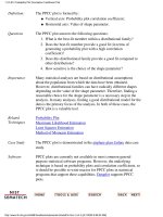
Importance:
Check
Distributional
Assumptions
Many statistical analyses, particularly in the field of reliability, are
based on the assumption that the data follow a Weibull distribution. If
the analysis assumes the data follow a Weibull distribution, it is
important to verify this assumption and, if verified, find good estimates
of the Weibull parameters.
Related
Techniques
Weibull Probability Plot
Weibull PPCC Plot
Weibull Hazard Plot
The Weibull probability plot (in conjunction with the Weibull PPCC
plot), the Weibull hazard plot, and the Weibull plot are all similar
techniques that can be used for assessing the adequacy of the Weibull
distribution as a model for the data, and additionally providing
estimation for the shape, scale, or location parameters.
The Weibull hazard plot and Weibull plot are designed to handle
censored data (which the Weibull probability plot does not).
Case Study
The Weibull plot is demonstrated in the airplane glass failure data case

study.
Software Weibull plots are generally available in statistical software programs
that are designed to analyze reliability data. Dataplot supports the
Weibull plot.
1.3.3.30. Weibull Plot
(2 of 3) [5/1/2006 9:57:09 AM]
1.3.3.30. Weibull Plot
(3 of 3) [5/1/2006 9:57:09 AM]