dohrmann Episode 2 Part 4 ppsx
Bạn đang xem bản rút gọn của tài liệu. Xem và tải ngay bản đầy đủ của tài liệu tại đây (643.08 KB, 10 trang )
“1
0.[1
0.6
exact
———
n=4
.—.—
n=8
1 2 3
4 5 6
7
8 9
10
‘2
Figure 14: Normalized shear stress 61~atcentroids of elements with edges on the slave boundary for mesh
configuration Q4Q4 (Case 2).
29
A Method for Connecting Dissimilar Finite Element
Meshes in Three Dimensions 1
C. R. Dohrmann2
S. W. Key3
M. W. Heinstein3
Abstract. A method is presented for connecting dissimilar finite element meshes in three
dimensions. The method combines the concept of master and slave surfaces with the uniform
strain approach for finite elements. By modifying the boundaries of elements on the slave
surface, corrections are made to element formulations such that first-order patch tests are
passed. The method can be used to connect meshes which use different element types.
In addition, master and slave surfaces can be designated independently of relative mesh
resolutions. Example problems in three-dimensional linear elasticity are presented.
Key Words. Finite elements, connected meshes, uniform strain, contact.
1Sandiais a multiprogramlaboratoryoperatedby SandiaCorporation,a LockheedMartinCompany,for
theUnitedStatesDepartmentof EnergyunderContractDE-AL0494AL8500.
2StructuralDynamicsDepartment,SandiaNationalLaboratories,MS0439,Albuquerque,NewMexico
87185-0439,email:crdohrmt%andia.gov,phone: (505) 8448058,fax: (505)844-9297.
3Engineeringand ManufacturingMechanicsDepartment,SandiaNationalLaboratories,MS0443,Albu-
querque,NewMexico87185-0443.
1. Introduction
In order to perform a finite element analysis, one may be required to connect two meshes
at a shared boundary.
Such requirements are common when assembling system models
from separate subsystem models. One approach to connecting the meshes requires that
both meshes have the same number of nodes, the same nodal coordinates, and the same
interpolation functions at the shared boundary. If these requirements are met, then the two
meshes can be connected simply by equating the degrees of freedom of corresponding nodes
at the shared boundary. As might be expected, connecting meshes in this manner often
requires a significant amount of time and effort in mesh generation.
An alternative to such an approach is to use the concept of “tied contact” to connect the
meshes. With this concept, one of the connecting mesh surfaces is designated as the master
surface and the other as the slave surface. For problems in solid mechanics, the meshes are
connected by constraining nodes on the slave surface to specific points on the master surface
at all times. Although this approach is appealing because of its simplicity, overlaps and gaps
may develop between the two meshes either because of non-planar initial geometry or non-
uniform displacements. For example, a node on the master surface may either penetrate or
pull away from the slave surface during deformation even though the slave node constraints
are all satisfied. As a result, displacement continuity may not hold at all locations on the
master-slave interface.
Several methods currently exist for connecting finite elements or meshes of elements.
Mesh grading approaches allow two or more finer elements to abut the edge of a neighbor-
ing coarser element [I]. Although such approaches generate conforming element boundaries,
they are not applicable to the general problem of connecting two dissimilar meshes. Other
methods [2-3] for connecting meshes based on constraint equations or Lagrange multiplier
approaches are applicable to a much broader class of problems, but they generally do not
ensure that mesh boundaries conform during deformation. Finite element approaches devel-
oped specifically for contact problems can also be used to connect meshes. These [4]include:
(i) Lagrange multiplier methods; (ii) penalty methods; and (iii) mixed methods. Many of
these methods are based in part on the master-slave concept.
Regardless of the method used to connect two meshes, it is important to address the
issues related to continuity at the mesh boundaries. One such issue is the first-order patch
test [5]. In general, meshes that are connected using existing methods based on constraint
equations or penalty functions alone fail the patch test. A general method for connecting
finite element meshes in two dimensions that passes the patch test was developed recently
by the authors [6]. This study investigates an extension of that method to three dimensions.
The basic idea is to redefine the boundaries of elements on the slave surface to achieve
a conforming connection with the master surface. The same idea was used recently at the
element level to obtain a conforming transition between hexahedral and tetrahedral elements
[7].
The present method combines the master-slave concept with the uniform strain approach
for finite elements [8]. As with the standard master-slave approach, nodes on the slave
surface are constrained to the master surface. In addition, the boundaries and formulations
1
of elements on the slave surface are modified to ensure that first-order patch tests are passed.
Consequently, results obtained using the method converge with mesh refinement.
A useful feature of the method is the freedom to designate the master and slave surfaces
independent ly of the resolutions of the two meshes. Standard practice commonly requires
the surface designated as the master to have fewer numbers of nodes than the slave surface.
The present method allows one to specify either of the mesh boundaries as master while still
satisfying the patch test. It is shown in Section 3 that improved accuracy can be achieved
in certain instantes by allowing the master surface to have the greater number of nodes.
Thus, there may be a preferred choice for the master surface in certain cases. Methods of
mesh refinement based on adaptive subdivision of existing elements may also benefit from
the method. For example, kinematic constraints on improper nodes could be removed while
preserving displacement continuity between adjacent elements.
Details of the method are presented in the following section. The presentation includes
a discussion of the uniform strain approach and the geometric concepts upon which the
method is based. Example problems in three-dimensional linear elasticity are presented in
Section 3. These examples highlight the various capabilities of the method. Comparisons
made with the standard master-slave approach demonstrate the superior performance of the
method.
2. Formulation
Consider a generic finite element in three dimensions with nodal coordinates xiI and nodal
displacements uzl for z = 1,2,3 and 1 = 1, ,
N. The spatial coordinates and displacements
of a point in the global coordinate direction ei are denoted by xi and ui, respectively.
isoparamet ric elements, the same interpolation functions are used for the coordinates
displacements. That is,
Xi = zil~~(ql, qz, ?73)
Ui = ual~l(?ll ,72, ~3)
For
and
(1)
(2)
where @I is the shape function of node 1 and (ql ,q2,q3) are isoparametric coordinates. A
summation over all possible values of repeated indices in Eqs. (1-2) and elsewhere is implied
unless noted otherwise.
The Jacobian determinant
J of the element is defined as
The volume
V of the element can be expressed in terms of J by
v=
J
JdV
Vq
(3)
(4)
where
Vq is the volume of integration of the element in the isoparametric coordinate system.
2
It is assumed that V is a homogeneous function of the nodal coordinates. It is also
assumed that a linear displacement field can be expressed exactly in terms of the shape
functions. Under these conditions, the uniform strain approach of Ref. 8 states that the
nodal forces jil associated with element stresses are given by
fzI = ~ijBjI
(5)
where Ozj are components of the
Cauchy stress tensor (~sumed constant thrwhout the
element), and
(6)
In addition, one has
V = xjIBjI for j = 1,2,3
(7)
where there is no summation over the index j in Eq. (7).
Closed-form expressions for Bjz are presented in Ref. 8 for the 8-node hexahedron- Similar
expressions can be derived for other element types, but they are quite lengthy for higher-
order elements. As an alternative to deriving closed-form expressions for specific element
types, one can use Gauss quadrature to determine Bjz for any
systematic manner.
By substituting Eqs. (1), (3) and (4) into Eq. (6), one finds
by the quadrature rule to evaluate Bjl are given by
isoparametric element in a
that the functions gjI used
911
= @I,l(~2,2~3,3 – ~3,2~2,3) + @Z,2(~2>3~3,1 – ~3,3~2,1) + h,3(~2,1~3,2 – ~3,1X2.2) (8)
921
= @I,l(~3,2%,3 – ~1,2~3,3) + @I,2(~3,3~l,l – ~1,3$3,1) + #Z,3(X3,1~l,2 – ~1,1~3,2) (9)
93: =
@I,l(~l,2z2,3 – ‘2,2X1,3) + #1,2(~1,3~2,1 – ~2,3~1,1) + @Z,3(~l,l~2,2 – ~2,1~1,2) (10)
and !gjz is evaluated at each of the quadrature points.
Exact values of
BjI can be obtained
using 2-point Gauss quadrature in three dimensions (8 quadrature points total) for the 8-
node hexahedron. For the 20-node serendipity or 27-node Lagrange hexahedron, 3-point
Gauss quadrature in three dimensions (27 quadrature points total) is required. Exact values
of
Bjz for the 4-node linear tetrahedron can be obtained using a l-point quadrature rule for
tetrahedral domains while the 10-node quadratic tetrahedron requires a 5-point quadrature
rule. Quadrature rules for integration over tetrahedral domains are available in Ref. 5.
Following the development in Ref. 8, one can show that
(13)
3
where fl is the domain of the element in the global coordinate system. Based on Eq. (13),
the uniform strain c“ of the element is expressed in terms of nodal displacements as
e‘=CU
(14)
where
and
u=
[
Ull U21
(16)
L
J
OBlZOO”””Bl~OO
o 0 B22 O “
0 B2N O
B~l O
0 B3z 0 0 B3N
O B22 B12 O ” B2N BIN O
B21 O B32 B22 0 B3N B2N
B1l B32 O B21 B3N
O BIN
1
T
u3~ u~2 U22 U32 . . . UIN U2N U3N
(17)
strain approach have the appealing feature that they passElements tm.wxlon the uniform
first-order patch tests.
Boundaries of three-dimensional elements are defined either by planar or curved faces.
Elements ~vith interpolation functions that vary linearly, e.g. the 4node tetrahedron, have
planar faces. In contrast, elements with higher-order interpolation functions, e.g. the 8-node
hexahedron and 10-node tetrahedron, generally have curved faces. That being the case, it
may not be otx~ious how to connect two meshes of elements which use different orders of
interpolation along their boundaries.
Difficulties can arise using the standard master-slave approach even if the boundaries of
both meshes are defined by planar faces.
As was mentioned previously, even though the
slave nodes stay attached to the master surface, there may not be any constraints to keep
a node on the master boundary from penetrating or pulling away from the slave boundary.
Such problems are addressed with the present method by requiring the faces of elements on
the slave boundary to always conform to the master boundary. In order to explain how this
is done. some preliminary geometric concepts are introduced first.
Notice from Eqs. (6), (14) and (16) that the relationship between strain and displacement
for a uniform strain element is defined completely by its volume. Consequently, the
uniform
strain
characteristics of two elements are identical if the expressions for their volumes are
the same. This fact is important because it allows one to consider alternative interpolation
functions for elements with faces on the master and slave surfaces. By doing so, one can
interpret the present method as an approach for generating “conforming” finite elements at
the shared boundary by carefully accounting for the volume (positive or negative) that exists
due to an imperfect match between the two meshes both initially and during deformation.
Consider an 8-node hexahedral element whose six faces are not necessarily planar. Each
point on a face of the element is associated with specific values of two isoparametric coor-
dinates. Both the spatial coordinates and displacements of the point are linear functions of
4
the coordinates and displacements of the four nodes defining the face. The specific forms of
these relationships are obtained by setting either ql, q2 or q3 equal to one of its bounding
values in Eqs. (1-2).
Consider now an alternative element in which each face of the original 8-node hexahedron
is triangulated with nt facets. Each vertex of a triangular facet intersects one of the curved
faces of the hexahedron. A center node c is introduced in the interior of the element.
Although the precise location of c is not important, its coordinates can be expressed in
terms of those of the hexahedron
The center node along with the
of a 4-node tetrahedron. Thus,
tetrahedral regions. Within each
as
(18)
three vertices of each triangular facet form the vertices
the domain of the hexahedron can be divided into 6nt
of these regions the interpolation functions are linear. In
other words, the displacement of a point in a tetrahedral region is determined by its location
and the displacements of the four nodes defining the tetrahedron. One may approximate the
boundary of the original hexahedron to any level of accuracy by increasing the number of
triangular facets.
Although the two elements described in the previous paragraphs are significantly dif-
ferent, their uniform strain characteristics are approximately the same. In the limit as nt
approaches infinity, the uniform strain characteristics of the two elements are identical. By
viewing all the element faces on the master and slave surfaces as connected triangular facets,
one can develop a systematic method for connecting the two meshes that passes first-order
patch tests. We note that the alternative element satisfies the basic assumptions of the
uniform strain approach.
That is, the element volume is a homogeneous function of the
nodal coordinates and a linear displacement field can be expressed exactly in terms of the
interpolation functions.
We are now in a position to present the method for modifying elements with faces on the
slave boundary. Changes to elements with faces on the master boundary are not required.
The concept of alternative piecewise-linear interpolation functions was introduced in the
previous paragraphs to facilitate interpretation of the method as a means for generating
conforming elements at the master-slave interface. These alternative interpolation functions
are never used explicitly to modify the element formulations.
Figure 1 depicts the projection of an element face F1 of the slave surface onto the master
surface. The larger filled circles designate nodes on the slave surface constrained to the
master surface. Smaller filled circles designate nodes on the master surface. Circles that are
not filled designate the projections of slave element edges onto master element edges.
Although there are several options for projecting slave element entities onto the master
surface, we opted for the following in this study. Nodes on the slave surface that are initially
off tl~e master surface are repositioned to specific points on the master surface based on a
minimum distance criterion. That is, a node on the slave surface is moved and constrained
to the nearest point on the master surface. For each element face of the slave surface, one
5
can define a normal direction at the center of the face. If an element edge of the slave surface
is shared by two elements, the normal direction for the edge is defined as the average of the
two elements sharing the edge. Otherwise, the normal direction is chosen as that of the
single element containing the edge. A plane is constructed which contains two nodes of the
slave element edge and has a normal in the direction of the cross product of the element
edge and the element edge normal. The projection of the slave element edge onto a master
element edge is simply the intersection of this plane with the master element edge.
Let P denote the element face of the master surface onto which a node S of the slave
surface is projected. The projection of S onto F’ can be characterized by two isoparametric
coordinate values qls and q2s. As a result of constraining S to P, the spatial coordinates of
S are expressed as
X~s = XaKa.Ks
(19)
where K ranges over all the nodes defining P.
The coefficient aKS in Eq. (19) can be
expressed in terms of qls and q2s by the equation
(20)
where ~~ is the shape function of node lS on face P.
The basic idea of the following development is to replace F’l with a new boundary which
prevents the possibility for overlaps or gaps between the two meshes. The new boundary is
composed of two parts. The first part is denoted by Fm and consists of the projection of F1
onto the master surface (see Figure 1). The second part is denoted by
FT and consists of
ruled surfaces between the edges of F’l and their projections onto the master surface. These
two parts of the new boundary are discussed in greater detail subsequently.
Using the divergence theorem, element volume can be expressed in terms of surface
integrals over the faces of the element as
(21)
where Nf is the number of element faces,
Fk denotes face k, and nk = n$ej is the unit
outward normal to ~k. Let V denote the volume of a uniform strain element obtained by
replacing
F1 with the new boundary. It follows from Eq. (21) that
v=v–
J
J
J
xjn~dS – ~ xjn~dS + ~ xjn~dS for j = 1,2,3
F1
m
r
(22)
where nn =
n~ej is the unit outward normal to
F~ and n’ = n~ej is the unit outward
normal to
F,. Notice that a negative sign is assigned to the third term on the right hand
side of Eq. (22) because n~ points into the slave element. The analog to Eq. (6) for the
uniform strain element is given by
7
(23)
6
The index~ is used instead of 1 in Eq. (23) to remind the reader that V depends on the
coordinates of the original element nodes as well as the nodes defining
F~. To be specific,
the index ~ takes on all values of 1 for the original element except the numbers of nodes
constrained to the master boundary. In addition, ~ takes on the numbers of all nodes defining
F
m.
Substituting Eqs. (19) and (22) into Eq. (23), one obtains
[ &(~Tx,n~ds-~,xjn~dS)
~j~ = Bj~ + ajs Bjs +
a
+—
u
/
xjn~ds – ~ xjn~dS
)
for j=l,2,3
~Xjf
F.
m
(24)
where the index S takes on the numbers of nodes constrained to the master boundary. Notice
that B,I = O if ~ refers to a node on the master boundary. In addition, CZISis zero if ~ refers
to node numbers of the original element. The terms involving surface integrals on the right
hand side Eq. (24) can be calculated using numerical integration as described in the following
paragraphs.
The coordinates of points on F1 can be expressed as
Xa= x~s~s(rll , qz)
(25)
where ~s is the shape function of node S on
F1. Using Eq. (25) and a fundamental result
for surface integrals, one obtains
where ‘$jkmis the permutation symbol and
Avl is the area of integration for
(26)
FI in the ql-q2
coordinate system.
Exact values of the integral on the right hand side of Eq. (26) can be
obtained using 2-point Gauss quadrature in two dimensions (4 quadrature points total) for
the 8-node hexahedron. For the 20-node and 27-node hexahedron, 3-point Gauss quadrature
in two dimensions (9 quadrature points total) is required. Exact values for the 4node
tetrahedron can be obtained using a l-point quadrature rule for triangular domains while
the 10-node tetrahedron requires a 7-point quadrature rule. Quadrature rules for integration
over triangular domains are available in Refs. 5 and 9.
The projection of F1 onto an element face of the master surface is shown in Figure 2. For
each such master element face, the boundary of the projection is defined by a closed polygon
consisting of straight-line segments in the isoparametric coordinate system of the master
element face. This polygon is decomposed into triangular regions (again in the isoparametric
coordinate system of the master element face) as shown to facilitate the calculation of surface
integrals.
The coordinates of points on the element face can be expressed as
Xa
= Zz&f@M(ql,qz)
(27)
7
where @M is the shape function for node M on the element
6’
J
ldS =Xj ?2j
/
~&f~jkmxk,l%z,2dA
dxjJ.f Flf Anf
face. From Eq. (27) one obtains
for j=l,2,3 (28)
where Flj denotes the projection of F1 onto the element face and
Aq~ is the area of integration
of the element face in the rj11-q2coordinate system.
The integral on the right hand side
of Eq. (28) is determined by adding the contributions from each triangular region. The
surface integrals can be calculated exactly for each triangular region by using the following
quadrature rules for triangular domains: l-point for 4-node tetrahedron, 4-point for 8-node
hexahedron, 7-point for 10-node tetrahedron, 13-point for 20-node hexahedron, and 19-point
for 27-node hexahedron. Surface integrals in Eq. (24) over the domain
F~ are obtained from
Eq. (28) by summing the contributions from all involved element faces on the master surface.
Recall that the second part of the boundary to replace
F1 consists of ruled surfaces
between the edges of
FI and their projections onto the master surface. These surfaces must
be considered only if the edges of
FI do not lie entirely on the master surface. By including
these surfaces, the “new boundary” of the slave element is ensured to be closed.
An edge of
F1 and its projection onto the master surface is shown in Figure 3. The spatial
coordinates of points along the edge can be expressed as
x~e= Xzs@se((2)
(29)
where q$s~is the shape function of node S on the edge of interest.
The projection of the edge onto a participating element face of the master surface appears
as one or more connected straight-line segments in the coordinate system of the element face.
For each such segment, the isoparametric coordinates of points along the segment can be
expressed as
L’1
= al + blfz
(30)
~2
=
a2 + b2{2 (31)
where the coefficients a and
b appearing in Eqs. (30-31) are determined from the projections
of nodes and edges of
F1 described previously. Thus, the spatial coordinates of points along
the segment can be expressed as
xi, =
xiM@M(al + bl~27 a2 + b2~2)
(32)
where @M is the shape function of node ~ on the element face.
The ruled surface between the segment and the edge is denoted by
Fg Spatial coordi-
nates of points on this surface are given by
Xz = (1 — ~l)~ig + ‘fIxie (33)
8