422 APPLIED COMPUTATIONAL FLUID DYNAMICS TECHNIQUES
where d
w
(x) is given by the Hermitian polynomial (Löhner (2001))
d
w
= 1 −3ξ
2
+ 2ξ
3
, (19.13)
and ξ is defined in (19.11). The final semi-discrete scheme takes the form
M
l
β
,t
= r =r
a
(u, v, β) + r
s
(d
w
,w)+ r
d
(d
h
,β), (19.14)
where the subscripts a, s and d stand for advection, source and damping. This system of
ODE’s is integrated in time using explicit time-marching schemes, e.g. a standard five-stage
Runge–Kutta scheme.
19.1.2. OVERALL SCHEME

One complete timestep consists of the following steps:
- given the boundary conditions for the pressure , update the solution in the 3-D fluid
mesh (velocities, pressures, turbulence variables, etc.);
- extract the velocity vector v =(u, v, w) at the free surface and transfer it to the 2-D
free surface module;
- given the velocity field, update the free surface β;
- transfer back the new free surface β to the 3-D fluid mesh, and impose new boundary
conditions for the pressure .
For steady-state applications, the fluid and free surface domains are updated using local
timesteps. This allows some room for variants that may converge faster to the final solution,
e.g. n steps of the fluid followed by m steps of the free surface, complete convergence of the
free surface between fluid updates, etc. Empirical evidence (Löhner et al. (1998, 1999a,c))
indicates that most of these variants prove unstable, or do not accelerate convergence
measurably. For steady-state applications it was found that an equivalent ‘time-interval’ ratio
between the fluid and the free surface of 1:8 yielded the fastest convergence (e.g. a Courant
number of C
f
= 0.25 for the fluid and C
s
= 2.0 for the free surface).
19.1.3. MESH UPDATE
Schemes that work with structured grids (e.g. Hino (1989,1997), Hino et al. (1993),
Farmer et al. (1993), Martinelli and Farmer (1994), Cowles and Martinelli (1996)) march the
solution in time until a steady state is reached. At each timestep, a volume update is followed
by a free surface update. The repositioning of points at each timestep implies a complete
recalculation of geometrical parameters, as well as interrogation of the CAD information
defining the surface. For general unstructured grids, this can lead to a doubling of CPU
requirements.For this reason, when solving steady-state problems,it is advisable not to move
the grid at each timestep, but only change the pressure boundary condition after each update
of the free surface β. The mesh is updated every 100 to 250 timesteps, thereby minimizing

the costs associated with geometry recalculations and grid repositioning along surfaces. One
can also observe that this strategy has the advantage of not moving the mesh unduly at the
beginning of a run, where large wave amplitudes may be present. One mesh update consists
of the following steps.
TREATMENT OF FREE SURFACES 423
- Obtain the new elevation for the points on the free surface from β. This only results in
a vertical (z-direction) displacement field d

for the boundary points.
- Apply the proper boundary conditions for the points on the waterline. This results in
an additional horizontal (x,y-direction) displacement field for the points on the water
line.
- Smooth the displacement field in order to avoid mesh distortion. This may be accom-
plished with any of the techniques described in Chapter 12.
- Interrogate the CAD data to reposition the points on the hull.
Denoting by d
∗
, n and t the predicted displacement of each point, surface normals and
tangential directions, the boundary conditions for the mesh movement are as follows (see
Figure 19.2).
x
z
y
a
d
b
b
b
e
c

c
f
g
a-f Hull, On Surface Patch
c-f Hull, End-Point
e-f Hull, Water Line End-Point In Plane of Symmetry
g
-f Water Surface Point in Plane of S
y
mmetr
y
b-f Hull, Line Point
d-f Hull, Water Line Point
f-f Water Surface Point
Figure 19.2. Boundary conditions for mesh movement
(a) Hull, on surface patch. The movement of these points has to be along the surface, i.e.
the normal component of d
∗
is removed:
d = d
∗
− (d
∗
· n) n. (19.15)
(b) Hull, line point. The movement of these points has to be along the lines, resulting in a
tangential boundary displacement of the form
d =(d
∗
· t)t. (19.16)
424 APPLIED COMPUTATIONAL FLUID DYNAMICS TECHNIQUES

(c) Hull, endpoint. No displacement is allowed for these points, i.e. d =0.
(d) Hull/water line point, water line endpoint. The displacement of these points is fixed,
given by the change in elevation z and the surface normal of the hull. Defining d
0
=
(0, 0,z),wehave
d =
d
0
− (d
0
· n) n
1 − n
2
z
. (19.17)
(e) Hull/water line endpoint in plane of symmetry. The displacement of these points is
fixed, and dictated by the tangential vector to the hull line in the symmetry plane:
d =
(d
0
· t)t
1 − n
2
t
. (19.18)
(f) Water surface points. These points start with an initial displacement d
0
, but may glide
along the water surface, allowing the mesh to accommodate the displacements in the

x,y-directions due to points on the hull. The normal to the water line is taken, and
(19.17) is used to correct any further displacements.
(g) Water surface points in plane of symmetry. As before, these points start with an initial
displacement d
0
, but may glide along the water surface, remaining in the plane of
symmetry, thus allowing the mesh to accommodate the displacements in the x-direction
due to points on the hull. The tangential direction is obtained from the sides lying on
the water surface in the plane of symmetry, and (19.18) is used to correct any further
displacements.
An option to restrict the movement of points completely in ‘difficult’ regions of the mesh
is often employed. Regions where such an option is required are transom sterns, as well as
the points lying in the half-plane given by the minimum z-value of the hull. Should negative
elements arise due to surface point repositioning, they are removed and a local remeshing
takes place. Naturally, these situations should be avoided as much as possible.
19.1.4. EXAMPLES FOR SURFACE FITTING
We include some examples that were computed using the algorithm outlined in the preceeding
sections. All of these consider the prediction of steady wave patterns for hulls over a wide
range of Froude numbers. For all of these cases, local timestepping was employed for the 3-D
incompressible flow solvers as well as the free surface solver. At the start of a run, the 3-D
flowfield was updated for 10 timesteps without any free surface update. Thereafter, the free
surface was updated after every 3-D flowfield timestep. The mesh was moved every 100 to
250 timesteps.
19.1.4.1. Submerged NACA0012
The first case considered is a submerged NACA0012 at α =5
◦
angle of attack. This same
configuration was tested experimentally by Duncan (1983) and modelled numerically by
Hino et al. (1993), Hino (1997). Although the case is 2-D, it was modelled as 3-D, with
two parallel walls in the y-direction. The mesh consisted of 2 409 720 tetrahedral elements,

TREATMENT OF FREE SURFACES 425
(a)
(b)
(c)
(d)
Figure 19.3. Submerged NACA0012: (a), (b) surface grids; (c), (d) pressure and velocity fields; (e),
(f) velocity field (zoom); (g) wave profiles
465752 points and 11 093 boundary points, of which 6929 were on the free surface. The
Froude number was set to Fr = 0.5672. This case was run in Euler mode and using the
Baldwin–Lomax model with a Reynolds number of Re = 10
6
. Figures 19.3(a)–(f) show the
surface grid, pressure and velocity fields, as well as a zoom of the velocity field close to
426 APPLIED COMPUTATIONAL FLUID DYNAMICS TECHNIQUES
(e)
(f)
-0.1
-0.08
-0.06
-0.04
-0.02
0
0.02
0.04
0.06
0.08
0.1
-2 -1 0 1 2 3 4 5
Wave Elevation (Fr=0.5672)
X-Coordinates

RANS
Euler
Hino 93
Experiment
(g)
Figure 19.3. Continued
the airfoil. Note the boundary layer from the velocity fields. Figure 19.3(g) compares the
wave profiles for the Euler, Baldwin–Lomax, Hino et al.’s (1993) Euler and Duncan’s (1983)
experiment data. The wave amplitudes are noticeably lower for the RANS case. Interestingly,
this was also observed by Hino (1997).
TREATMENT OF FREE SURFACES 427
19.1.4.2. Wigley hull
The next case is the well-known Wigley hull, given by the analytical formula
y = 0.5 ·B ·[1 −4x
2
]·

1 −

z
D

2

, (19.19)
where B and D are the beam and the draft of the ship at still water. For the case considered
here, D = 0.0625 and B =0.1. This same configuration was tested experimentally at the
University of Tokyo (ITTC (1983a,b)) and modelled numerically by Farmer et al. (1993),
Raven (1996) and others. At first, a fine triangulation for the surface given by (19.19) was
generated. This triangulation was subsequently used to define, in a discrete manner, the hull.

The surface definition of the complete computational domain consisted of discrete (hull) and
analytical surface patches. The mesh consisted of 1119703 tetrahedral elements, 204155
points and 30358 boundary points, of which 15 515 were on the free surface. The parameters
for this simulations were as follows: Fr = 0.25, Re = 10
6
and the k −  model with the law
of the wall approximation. Figures 19.4(a) and (b) show the surface grids employed, and
the extent of the region with high-aspect-ratio elements. In Figures 19.4(c) and (d) the wave
profiles and surface velocities obtained from Euler and RANS calculations are compared. As
expected, the effect of viscosity becomes noticeable in the stern region. Figure 19.4(e) shows
the comparison to the experiments conducted at the University of Tokyo. It can be noticed
that the first wave is accurately reproduced, but that the second wave is not well reproduced
by the calculations.
19.1.4.3. Double Wigley hull
The third case considered is an inviscid case comprising two Wigley hulls positioned close
to each other. Figures 19.5(a)–(f) show the resulting wave pattern for a Froude number of
Fr = 0.316 for different relative spacings in the x-andy-directions. As one can see, the
effect on the resulting wave pattern is considerable.
19.1.4.4. Wigley carrier group
The next case considered is again inviscid. The configuration is composed of a Wigley hull
in the centre that has been enlarged by a factor of 1:3, surrounded by normal Wigley hulls.
The mesh consisted of approximately 4.2 million tetrahedra. Figures 19.6(a) and (b) show the
resulting wave pattern for a Froude number of Fr = 0.316. The CPU time for this problem
was approximately 24 hours using eight processors on an SGI Origin2000.
19.1.5. PRACTICAL LIMITATIONS OF FREE SURFACE FITTING
While very accurate and extremely competitive in terms of storage and CPU requirements as
compared to other methods, free surface fitting also has limitations. The key limitation stems
from the free surface description given by (19.4). Any free surface described in this manner
can only be single-valued in the z-direction. Therefore, it will be impossible to describe a
breaking wave. Another case where this method fails is the situation where transom sterns

have vertical walls. Here, as before, the free surface becomes multi-valued. Summarizing,
free surface fitting methods cannot be used if the interface topology changes significantly.
428 APPLIED COMPUTATIONAL FLUID DYNAMICS TECHNIQUES
(a) (b)
Euler RANS (kŦH)
Euler RANS (kŦH)
(c) (d)
-0.006
-0.004
-0.002
0
0.002
0.004
0.006
0.008
0.01
0.012
0.014
-1 -0.8 -0.6 -0.4 -0.2 0 0.2 0.4 0.6 0.8 1
Wave Elevation (Fr=0.25)
X-Coordinates
RANS
Euler
Experiment
(e)
Figure 19.4. Wigley hull: (a), (b) surface of mesh; (c) wave elevation; and (d) surface velocity; (e) wave
elevation at the hull
TREATMENT OF FREE SURFACES 429
dx=0.10, dy=0.50 dx=0.25, dy=0.50 dx=0.50, dy=0.50
(a)

(b) (c)
dx=0.10, dy=0.25 dx=0.25, dy=0.25 dx=0.50, dy=0.25
(d)
(e)
(f)
Figure 19.5. (a)–(c) Wave elevation for two Wigley hulls (Fr = 0.316); (d)–(f) wave elevation for two
Wigley hulls (Fr =0.316)
19.2. Interface capturing methods
As stated before, the third possible approach to treat free surfaces is given by the so-
called interface-capturing methods (Nichols and Hirt (1975), Hirt and Nichols (1981),
Yabe and Aoki (1991), Unverdi and Tryggvason (1992), Sussman et al. (1994), Yabe (1997),
430 APPLIED COMPUTATIONAL FLUID DYNAMICS TECHNIQUES
(a)
(b)
Figure 19.6. (a) Wigley carrier group; (b) wave elevation (Fr =0.316)
TREATMENT OF FREE SURFACES 431
Scardovelli and Zaleski (1999), Chen and Kharif (1999), Fekken et al. (1999), Enright et al.
(2003), Biausser et al. (2004), Huijsmans and van Grosen (2004),Coppola-Owen and Codina
(2005)). These consider both fluids as a single effective fluid with variable properties; the
interface is captured as a region of sudden change in fluid properties. The main problem
of complex free surface flows is that the density ρ jumps by three orders of magnitude
between the gaseous and liquid phases. Moreover, this surface can move, bend and reconnect
in arbitrary ways. In order to illustrate the difficulties that can arise if one treats the complete
system, consider a hydrostatic flow, where the exact solution is v = 0,p=−ρg · (x − x
0
),
and x
0
denotes the position of the free surface. Unless the free surface coincides with the
faces of elements, there is no way for typical finite element shape functions to capture the

discontinuity in the gradient of the pressure. This implies that one has to either increase the
number of Gauss points (Codina and Soto (2002)) or modify (e.g. enrich) the shape function
space (Coppola-Owen and Codina (2005), Kölke (2005)). Using the standard linear element
procedure leads to spurious velocity jumps at the interface, as any small pressure gradient
that ‘pollutes over’ from the water to the air region will accelerate the air considerably. This
in turn will lead to loss of divergence, causing more spurious pressures. The whole cycle may,
in fact, lead to a complete divergence of the solution. Faced with this dilemma, most flows
with free surfaces have been solved neglecting the air. This approach does not account for the
pressure buildup due to volumes of gas enclosed by liquid, and therefore is not universal.
The liquid–gas interface is described by a scalar equation of the form

,t
+ v
a
·∇ = 0. (19.20)
For the classic volume of fluid (VOF) technique,  represents the percentage of liquid in
a cell/element or control volume (see Nichols and Hirt (1975), Hirt and Nichols (1981),
Scardovelli and Zaleski (1999), Chen and Kharif (1999), Fekken et al. (1999), Biausser et al.
(2004), Huijsmans and van Grosen (2004)). For pseudo-concentration (PC) techniques, 
represents the total density of the material in a cell/element or control volume. For the level
set (LS) approach  represents the signed distance to the interface (Enright et al. (2003)).
One complete timestep for a projection-based incompressible flow solver as described in
Chapter 11 then comprises of the following substeps:
- predict velocity (advective-diffusive predictor, equations (11.32a), (11.41) and
(11.42));
- extrapolate the pressure (imposition of boundary conditions);
- update the pressure (equation (11.32b));
- correct the velocity field (equation (11.32c));
- extrapolate the velocity field; and
- update the scalar interface indicator.

The extension of a solver for the incompressible Navier–Stokes equations to handle free
surface flows via the VOF or LS techniques requires a series of extensions which are the
subject of the present section. At this point, we remark that the implementation of the VOF
and LS approaches is very similar. Moreover, experience indicates that both work well.
432 APPLIED COMPUTATIONAL FLUID DYNAMICS TECHNIQUES
p
p
p=p
g
p=p
g
p=p
g
p
p
Liquid
Interface
Gas
p
p
p
p
p
p
Interface
v
v
v
Layer 1
Layer 2

Gas
Liquid
v
(a) (b)
Figure 19.7. Extrapolation of (a) the pressure and (b) the velocity
For VOF, it is important to have a monotonicity preserving scheme for .ForLS,itis
important to balance the cost and accuracy loss of re-initializations vis-à-vis propagation. In
what follows, we will assume that  is bounded by values for liquid and gas (e.g. 0 ≤  ≤1
for VOF, ρ
g
≤  ≤ ρ
l
for PC) and that the liquid–gas interface is defined by the average of
these extreme values (i.e.  = 0.5forVOF, = 0.5 · (ρ
g
+ ρ
l
) for PC,  =0forLS).
19.2.1. EXTRAPOLATION OF THE PRESSURE
The pressure in the gas region needs to be extrapolated in order to obtain the proper velocities
in the region of the free surface. This extrapolation is performed using a three-step procedure.
In the first step, the pressures for all points in the gas region are set to (constant) values,
either the atmospheric pressure or, in the case of bubbles, the pressure of the particular
bubble. In a second step, the gradient of the pressure for the points in the liquid that are
close to the liquid–gas interface are extrapolated from the points inside the liquid region
(see Figure 19.7(a)). This step is required as the pressure gradient for these points cannot be
computed properly from the data given. Using this information (i.e. pressure and gradient of
pressure), the pressure for the points in the gas that are close to the liquid–gas interface are
computed.
19.2.2. EXTRAPOLATION OF THE VELOCITY

The velocity in the gas region needs to be extrapolated properly in order to propagate
accurately the free surface. This extrapolation is started by initializing all velocities in the gas
region to v =0. Then, for each subsequent layer of points in the gas region where velocities
have not been extrapolated (unknown values), an average of the velocities of the surrounding
points with known values is taken (see Figure 19.7(b)).
19.2.3. KEEPING INTERFACES SHARP
The VOF and PC options propagate Heavyside functions through an Eulerian mesh. The
‘sharpness’ of such profiles requires the use of monotonicity-preserving schemes for advec-
tion, such as total variation diminishing (TVD) or flux-corrected transport (FCT) techniques
TREATMENT OF FREE SURFACES 433
(see Chapters 9 and 10). LS methods propagate a linear function, which numerically is a
much simpler problem. Regardless of the technique used, one finds that shear and vortical
flowfields will tend to smooth and distort . Fortunately, both TVD and FCT algorithms
allow for limiters that keep the solution monotonic while enhancing the sharpness of the
solution. For the TVD schemes Roe’s Super-B limiter (Sweby (1984)) produces the desired
effect. For FCT one increases the anti-diffusion by a small fraction (e.g. c = 1.01). The
limiting procedure keeps the solution monotonic, while the increased anti-diffusion steepens
 as much as is possible on a mesh. With these schemes, the discontinuity in  is captured
within one to two gridpoints for all times. For LS the distance function  must be reinitialized
periodically so that it truly represents the distance to the liquid–gas interface. The increase of
CPU requirements can be kept to a minimum by using fast marching techniques and proper
data structures (see Chapter 2, as well as Sethian (1999) and Osher and Fedkiw (2002)).
19.2.4. IMPOSITION OF CONSTANT MASS
Experience indicates that the amount of liquid mass (as measured by the region where the
VOF indicator is larger than a cut-off value) does not remain constant for typical runs.
The reasons for this loss or gain of mass are manifold: loss of steepness in the interface
region, inexact divergence of the velocity field, boundary velocities, etc. This lack of exact
conservation of liquid mass has been reported repeatedly in the literature (Sussman et al.
(1994), Sussman and Puckett (2000), Enright et al. (2003)). The classic recourse is to
add/remove mass in the interface region in order to obtain an exact conservation of mass. At

the end of every timestep, the total amount of fluid mass is compared to the expected value.
The expected value is determined from the mass at the previous timestep, plus the mass flux
across all boundaries during the timestep. The differences in expected and actual mass are
typically very small (less than 10
−4
), so that quick convergence is achieved by simply adding
and removing mass appropriately. The key question is where to add and remove mass. A
commonly used approach is to make the mass taken/added proportional to the absolute value
of the normal velocity of the interface:
v
n
=




v ·
∇
|∇|




. (19.21)
In this way the regions with no movement of the interface remain unaffected by the changes
made to the interface in order to impose strict conservation of mass. The addition and removal
of mass typically occurs at points close to the liquid–gas interface, where  does not assume
extreme values. In some instances, the addition or removal of mass can lead to values of 
outside the allowed range. If this occurs, the value is capped at the extreme value, and further
corrections are carried out at the next iteration.

19.2.5. DEACTIVATION OF AIR REGION
Given that the air region is not treated/updated, any CPU spent on it may be considered
wasted. Most of the work is spent in loops over the edges (upwind solvers, limiters, gradients,
etc.). Given that edges have to be grouped in order to avoid memory contention/allow
vectorization when forming RHSs (see Chapter 15), this opens a natural way of avoiding
434 APPLIED COMPUTATIONAL FLUID DYNAMICS TECHNIQUES
Air
Free Surface
Bubble
Figure 19.8. Bubble in water
unnecessary work: form relatively small edge groups that still allow for efficient vectoriza-
tion, and deactivate groups instead of individual edges (see Chapter 16). In this way, the basic
loops over edges do not require any changes. The if-test for whether an edge group is active
or deactive occurs outside the inner loops over edges, leaving them unaffected. On scalar
processors, edge groups as small as negrp=8 may be used. Furthermore,if points and edges
are grouped together in such a way that proximity in memory mirrors spatial proximity, most
of the edges in air will not incur any CPU penalty.
19.2.6. TREATMENT OF BUBBLES
The treatment of bubbles follows the classic assumption that the timescales associated with
the speed of sound in the bubble are much faster than the timescales of the surrounding fluid.
This implies that at each instance the pressure in the bubble is (spatially) constant. As long
as the bubble is not in contact with the atmospheric air (see Figure 19.8), the pressure can be
obtained from the isentropic relation
p
b
p
b0
=

ρ

b
ρ
b0

γ
, (19.22)
where p
b
,ρ
b
denote the pressure and density in the bubble and p
b0
and ρ
b0
the reference
values (e.g. those at the beginning of the simulation). The gas in the bubble is marked by
solving a scalar advection equation of the form given by (19.20):
b
,t
+ v
a
·∇b =0, (19.23)
where, initially, b = 1.0 denotes the bubble region and b =0.0 the remainder of the flowfield.
The same advection schemes and steepening algorithms as used for  are also used for b.
At the beginning of every timestep the total volume occupied by the gas is added. From this
volume the density is inferred, and the pressure is computed from (19.22).
At the end of every timestep, a check is performed to see whether the bubble has reached
contact with the air. This happens if we have, at a given point, b>0.5and>
0.5
. Should

this be the case, the neighbour elements of these points that are in air are set to b =1.0. This
increases the volume occupied by the bubble, thereby reducing the pressure. Over the course
of a few timesteps, the pressure in the bubble then reverts to atmospheric pressure, and one
observes a rather quick bubble collapse.
TREATMENT OF FREE SURFACES 435
19.2.7. ADAPTIVE REFINEMENT
As seen in Chapter 14, adaptive mesh refinement may be used to reduce CPU and memory
requirements without compromising the accuracy of the numerical solution. For multiphase
problems the mesh can be refined automatically close to the liquid–gas interface (Hay and
Visonneau (2005), Löhner et al. (2006)). This may be done by including two additional
refinement indicators (in addition to the usual ones based on the flow variables). The first one
looks at the edges cut by the liquid–gas interface value of , and refines the mesh to a certain
element size or refinement level (Löhner and Baum (1992)). The second, more sophisticated
indicator, looks at the liquid–gas interface curvature, given by
κ =∇·n, n =
∇
|∇|
, (19.24)
and refines the mesh only in regions where the element size is deemed insufficient.
19.2.8. EXAMPLES FOR SURFACE CAPTURING
19.2.8.1. Breaking dam problem
This is a classic test case for free surface flows. The problem definition is shown in
Figure 19.9(a). This case was run on a coarse mesh with nelem=16,562 elements, a fine
mesh with nelem=135,869 and an adaptively refined mesh (where the coarse mesh was
the base mesh) with approximately nelem=30,000 elements. The refinement indicator for
the latter was the free surface (see above), and the mesh was adapted every five timesteps.
Figure 19.9(b) shows the discretization for the coarse mesh, and Figures 19.9(c)–(f) the
development of the flowfield and the free surface until the column of water hits the right
wall. Note the mesh adaptation in time. The results obtained for the horizontal location of
the free surface along the bottom wall are compared to the experimental values of Martin and

Moyce (1952), as well as the numerical results obtained by Hansbo (1992), Kölke (2005) and
Walhorn (2002) in Figure 19.9(g). The dimensionless time and displacement are given by
τ = t
√
2g/a and δ = x/a,wherea is the initial width of the water column. As one can see,
the agreement is very good, even for the coarse mesh. The difference between the adaptively
refined mesh and the fine mesh was almost indistinguishable, and therefore only the results
for the fine mesh are shown in the graph.
19.2.8.2. Sloshing of a 2-D tank due to sway excitation
This example, taken from Löhner (2006), considers the sloshing of a partially filled 2-D
tank. The main tank dimensions are L = H = 1 m, with tank width B = 0.1 m. The problem
definition is shown in Figure 19.10(a). Experimental data for this tank with a filling level
h/L = 0.35 have been provided by Olsen (1970), and reported in Faltisen (1974) and Olsen
and Johnsen (1975), where the tank was undergoing a sway motion, i.e. the tank oscillates
horizontally with law x =A sin(2πt/T). A wave gauge was placed0.05 m fromtheright wall
and the maximum wave elevation relative to a tank-fixed coordinate system was recorded. In
the numerical simulations reported by Landrini et al. (2003) using the SPH method,theforced
oscillation amplitude increases smoothly in time and reaches its steady regime value in 10 T.
436 APPLIED COMPUTATIONAL FLUID DYNAMICS TECHNIQUES
14.0
7.0
3.5
10.0
U 
P  g=(0,-1,0)
(a) (b)
(c) (d)
(e) (f)
Figure 19.9. Breaking dam: (a) problem definition; (b) surface discretization for the coarse mesh;
(c)–(f) flowfield at different times; (g) horizontal displacement

The simulation continues for another 30 T and the maximum wave elevation is recorded in
the last 10 periods of oscillation.
The same procedure as in Landrini et al. (2003) was followed for the 32 cases computed.
This corresponds to two amplitudes(A = 0.025, 0.05) and 16 periods, in the range T =1.0 −
1.8sorT/T
1
= 0.787–1.42, where T
1
= 1.27 s. When h/L = 0.35 the primary resonances
of the first and the third modes occur at T/T
1
= 1.0andT/T
1
= 0.55, respectively. The
secondary resonance of the second mode is at T/T
1
= 1.28 (see Landrini et al. (2003)).
The VOF results for the time history of the lateral force F
x
when T = 1.2, 1.3and
TREATMENT OF FREE SURFACES 437
1.0
1.5
2.0
2.5
3.0
3.5
4.0
0.0 0.5 1.0 1.5 2.0 2.5 3.0
dimensionless displacement

dimensionless time
Martin/Moyce
Hansbo
Walhorn
Sauer
Koelke
FEFLO Coar
FEFLO Fine
(g)
Figure 19.9. Continued
Y
L=1m
H=1m
A1
50mm
A
h=0.35m
X
(a)
Figure 19.10. 2-D tank: (a) problem definition; (b) time history of lateral force F
x
; (c) time history of
wave elevation (probe A1); (d) snapshots of free surface wave elevation for T = 1.3andA/L = 0.05;
(e) maximum wave height (probe A1); (f), (g) maximum absolute values of lateral force F
x
for A/L =
0.025, 0.05
A = 0.025, 0.05 are shown in Figure 19.10(b). The corresponding time history of the wave
elevation at the wave probe A1 (see Figure 19.10(a)) are shown in Figure 19.10(c). Some
free surface snapshots are shown in Figure 19.10(d). The dark line represents the free

438 APPLIED COMPUTATIONAL FLUID DYNAMICS TECHNIQUES
-150
-100
-50
0
50
100
150
0 5 10 15 20 25 30 35 40
F
x
10
3
/ρ gL
2
b
t/T
VOF, T 1.2, A/L 0.025
-150
-100
-50
0
50
100
150
0 5 10 15 20 25 30 35 40
F
x
10
3

/ρ gL
2
b
t/T
VOF, T 1.2, A/L 0.05
-150
-100
-50
0
50
100
150
0 5 10 15 20 25 30 35 40
F
x
10
3
/ρ gL
2
b
t/T
VOF, T 1.3, A/L 0.025
-150
-100
-50
0
50
100
150
0 5 10 15 20 25 30 35 40

F
x
10
3
/ρ gL
2
b
t/T
VOF, T 1.3, A/L 0.05
(b)
-0.6
-0.4
-0.2
0
0.2
0.4
0.6
0 5 10 15 20 25 30 35 40
wave elevation (ζ /L)
t/T
VOF, T 1.2, A/L 0.025
-0.6
-0.4
-0.2
0
0.2
0.4
0.6
0 5 10 15 20 25 30 35 40
wave elevation (ζ /L)

t/T
VOF, T 1.2, A/L 0.05
-0.6
-0.4
-0.2
0
0.2
0.4
0.6
0 5 10 15 20 25 30 35 40
wave elevation (ζ /L)
t/T
VOF, T 1.3, A/L 0.025
-0.6
-0.4
-0.2
0
0.2
0.4
0.6
0 5 10 15 20 25 30 35 40
wave elevation (ζ /L)
t/T
VOF, T 1.3, A/L 0.05
(c)
Figure 19.10. Continued
surface. Note also the ‘undershoots’ in the pressure due to extrapolation. The VOF results
for maximum wave elevation ζ at the wave probe A1 (see Figure 19.10(a)) are compared
with the experimental data and SPH results (Landrini et al. (2003)) in Figure 19.10(e) for
A/L =0.025, 0.05. Note that, as the wave inclination close to the wall is considerable, there

is a non-negligible uncertainty in both the experiments and computational results.
The predicted lateral absolute values of maximum forces are compared with the exper-
imental data and SPH results (Landrini et al. (2003)) in Figure 19.10(f) for A/L = 0.05.
Figure 19.10(g) shows the comparisonof predicted lateral absolute values of maximum forces
for A/L = 0.025, 0.05. It canbe seen fromFigures19.10(e)–(g)thatboth the maximum wave
height and lateral absolute values of maximum forces predicted by the present VOF method
TREATMENT OF FREE SURFACES 439
(d)
Figure 19.10. Continued
agree fairly well with the experimental data and SPH results, with a small phase shift among
the three results. Figures 19.10(b) and (c) are typical time history plots. It should be noted
from these figures that, even after a long simulation time (40 periods), steady-state results are
not generally obtained. This is due to very small damping in the system. Landrini et al. (2003)
noted the same behaviour in their numerical simulations. As a result, the predicted maximum
wave elevation and the lateral absolute values of maximum forces plotted in Figure 19.10(e)
are average maximum values for the last few periods for the cases when the steady state is
not reached.
19.2.8.3. Sloshing of a 3-D tank due to sway excitation
In order to study the 3-D effects, the sloshing of a partially filled 3-D tank is considered. The
main tank dimensions are L = H = 1 m, with tank width b =1 m. The problem definition is
shown in Figure 19.11(a). The 3-D tank has the same filling level h/L = 0.35 as the 2-D tank.
The 3-D tank case is run on a mesh with nelem=561,808 elements, and the 2-D tank is
run on a mesh with nelem=54,124 elements. The numerical simulations are carried out for
both 3-D and 2-D tanks, where both tanks are undergoing the same prescribed sway motion
440 APPLIED COMPUTATIONAL FLUID DYNAMICS TECHNIQUES
0
0.1
0.2
0.3
0.4

0.5
0.6
0.7
0.7 0.8 0.9 1 1.1 1.2 1.3 1.4 1.5
wave height (ζ /L)
T/T
1
VOF, A/L 0.025
Exp, A/L 0.025
SPH, A/L 0.025
0
0.1
0.2
0.3
0.4
0.5
0.6
0.7
0.7 0.8 0.9 1 1.1 1.2 1.3 1.4 1.5
wave height (ζ /L)
T/T
1
VOF, A/L 0.05
Exp, A/L 0.05
SPH, A/L 0.05
(e)
0
20
40
60

80
100
120
140
160
180
0.7 0.8 0.9 1 1.1 1.2 1.3 1.4 1.5
F
x
10
3
/U gL
2
b
T/T
1
VOF, A/L=0.05
Exp, A/L=0.05
SPH, A/L=0.05
0
20
40
60
80
100
120
140
160
180
0.7 0.8 0.9 1 1.1 1.2 1.3 1.4 1.5

F
x
10
3
/U gL
2
b
T/T
1
VOF, A/L=0.050
VOF, A/L=0.025
(f) (g)
Figure 19.10. Continued
L1m
H1m
X
h 0.35m
Y
AB1m
Z
(a)
Figure 19.11. 3-D tank: (a) problem definition; time history of force F
x
for (b) a 2-D tank and (c) a 3-D
tank at A/L = 0.025,T/T
1
= 1; (d) time history of force F
z
for a 3-D tank at A/L = 0.025,T/T
1

= 1;
(e), (f), (g) snap shots of the free surface wave elevation for a 3-D tank
TREATMENT OF FREE SURFACES 441
-150
-100
-50
0
50
100
150
0 10 20 30 40 50 60 70 80
F
x
10
3
/ρ gL
2
b
t/T
VOF, A/L 0.025, 2D Tank
(b)
-150
-100
-50
0
50
100
150
0 10 20 30 40 50 60 70 80
F

x
10
3
/ρ gL
2
b
t/T
VOF, A/L 0.025, 3D Tank
(c)
-150
-100
-50
0
50
100
150
0 10 20 30 40 50 60 70 80
F
z
10
3
/ρ gL
2
b
t/T
VOF, A/L 0.025, 3D Tank
(d)
Figure 19.11. Continued
given by x = A sin(2πt/T). The simulations were carried out for A = 0.025 and T = 1.27
(i.e. T/T

1
= 1). The forced oscillation amplitude increases smoothly in time and reaches its
steady regime value in 10 T. The simulation continues for another 70 T. In order to show
the 3-D effects, the forces are non-dimensionalized with ρgL
2
b for both 2-D and 3-D tanks.
Figures 19.11(b) and (c) show the time history of the force F
x
(horizontal force in the same
direction as the tank moving direction) for both 2-D and 3-D tanks. Figure 19.11(d) shows
the time history of the force F
z
(horizontal force perpendicular to the tank moving direction)
for the 3-D tank. It is very interesting to observe from Figures 19.11(c) and (d) that there are
442 APPLIED COMPUTATIONAL FLUID DYNAMICS TECHNIQUES
(e)
Figure 19.11. Continued
TREATMENT OF FREE SURFACES 443
(f)
Figure 19.11. Continued
444 APPLIED COMPUTATIONAL FLUID DYNAMICS TECHNIQUES
(g)
Figure 19.11. Continued
TREATMENT OF FREE SURFACES 445
245.7m
310m
120m
700m
x=x0+a sin( t)
y

z
x
Z
(a)
(b)
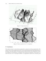
Figure 19.12. Ship adrift: (a) problem definition; (b) evolution of the free surface; (c), (d): position of
center of mass; (e) roll angle versus time
446 APPLIED COMPUTATIONAL FLUID DYNAMICS TECHNIQUES
-40
-20
0
20
40
60
80
100
120
0 20 40 60 80 100 120 140 160 180 200 220
Position
Time
x_c
-5
0
5
10
15
20
25
30
35

-40 -20 0 20 40 60 80 100 120
z-Position
x-Position
x_c vs z_c
(c) (d)
-0.15
-0.1
-0.05
0
0.05
0.1
0.15
0.2
0 20 40 60 80 100 120 140 160 180 200 220
Angle
Time
a_x
(e)
Figure 19.12. Continued
almost no 3-D effects for the first 25 oscillating periods. The 3-D modes start to appear after
25 T, and fully build up at about 40 T. The 3-D flow pattern then remains steady and periodic
for the rest of the simulation, which is about 40 more oscillation periods.
Figures 19.11(e)–(g) show a sequence of snapshots of the free surface wave elevation for
the 3-D tank. For the first set of snapshots (see Figure 19.11(e)), the flow is still 2-D. The
3-D flow starts to build up in the second set of snapshots (see Figure 19.11(f)). The flow
remains periodic 3-D for the last 40 periods. Figure 19.11(g) shows typical snapshots of the
free surface for the last 40 periods. The 3-D effects are clearly shown in these plots.
19.2.8.4. Drifting ship
This example shows the use of interface capturing to predict the effects of drift in waves for
large ships. The problem definition is given in Figure 19.12(a). The ship is a generic liquefied

natural gas (LNG) tanker, and is considered rigid. The waves are generated by moving the
left wall of the domain. A large element size was specified at the far end of the domain in
order to dampen the waves. The mesh at the ‘wave-maker plane’ is moved using a sinusoidal
excitation. The ship is treated as a free, floating object subject to the hydrodynamic forces
of the water. The surface nodes of the ship move according to a 6-DOF integration of the
rigid-body motion equations. Approximately 30 layers of elements close to the ‘wave-maker