Fiber Optic Telecommunication phần 2 pps
Bạn đang xem bản rút gọn của tài liệu. Xem và tải ngay bản đầy đủ của tài liệu tại đây (909.98 KB, 10 trang )
F
IBER
O
PTIC
T
ELECOMMUNICATION
© 2000 University of Connecticut 303
2
N.A.
a
V
π
λ
=×
(8-5)
or by Equation 8-6.
V
a
n=×××
2
2
1
1
2
π
λ
∆
a
f
(8-6)
In either equation, a is the fiber core radius, λ is the operating wavelength, N.A. is the
numerical aperture, n
1
is the core index, and ∆ is the relative refractive index difference between
core and cladding.
The analysis of how the V-number is derived is beyond the scope of this module, but it can be
shown that by reducing the diameter of the fiber to a point at which the V-number is less than
2.405, higher-order modes are effectively extinguished and single-mode operation is possible.
Example 4
What is the maximum core diameter for a fiber if it is to operate in single mode at a wavelength of
1550 nm if the N.A. is 0.12?
From Equation 8-5,
2
N.A.
a
V
π
λ
=×
Solving for
a
yields
a
= (
V
)(
λ
)/(2
π
N.A.)
For single-mode operation,
V
must be 2.405 or less. The maximum core diameter occurs when
V
= 2.405. So, plugging into the equation, we get
a
max
= (2.405)(1550 nm)/[(2
π
)(0.12)] = 4.95
µ
m
or
d
max
= 2
×
a
= 9.9
µ
m
The core diameter for a typical single-mode fiber is between 5 µm and 10 µm with a 125-µm
cladding. Single-mode fibers are used in applications in which low signal loss and high data
rates are required, such as in long spans where repeater/amplifier spacing must be maximized.
Because single-mode fiber allows only one mode or ray to propagate (the lowest-order mode), it
does not suffer from modal dispersion like multimode fiber and therefore can be used for higher
bandwidth applications. However, even though single-mode fiber is not affected by modal
dispersion, at higher data rates chromatic dispersion can limit the performance. This problem
can be overcome by several methods. One can transmit at a wavelength in which glass has a
fairly constant index of refraction (~1300 nm), use an optical source such as a distributed-
feedback laser (DFB laser) that has a very narrow output spectrum, use special dispersion-
F
UNDAMENTALS OF
P
HOTONICS
304 © 2000 University of Connecticut
compensating fiber, or use a combination of all these methods. In a nutshell, single-mode fiber
is used in high-bandwidth, long-distance applications such as long-distance telephone trunk
lines, cable TV head-ends, and high-speed local and wide area network (LAN and WAN)
backbones. The major drawback of single-mode fiber is that it is relatively difficult to work with
(i.e., splicing and termination) because of its small core size. Also, single-mode fiber is typically
used only with laser sources because of the high coupling losses associated with LEDs.
Graded-index fiber is a compromise between the large core diameter and N.A. of multimode
fiber and the higher bandwidth of single-mode fiber. With creation of a core whose index of
refraction decreases parabolically from the core center toward the cladding, light traveling
through the center of the fiber experiences a higher index than light traveling in the higher
modes. This means that the higher-order modes travel faster than the lower-order modes, which
allows them to “catch up” to the lower-order modes, thus decreasing the amount of modal
dispersion, which increases the bandwidth of the fiber.
VI. D
ISPERSION
Dispersion, expressed in terms of the symbol ∆t, is defined as pulse spreading in an optical
fiber. As a pulse of light propagates through a fiber, elements such as numerical aperture, core
diameter, refractive index profile, wavelength, and laser linewidth cause the pulse to broaden.
This poses a limitation on the overall bandwidth of the fiber as demonstrated in Figure 8-3.
Figure 8-3 Pulse broadening caused by dispersion
Dispersion ∆t can be determined from Equation 8-7.
∆t = (∆t
out
– ∆t
in
)
1
/
2
(8-7)
and is measured in time, typically nanoseconds or picoseconds. Total dispersion is a function of
fiber length. The longer the fiber, the more the dispersion. Equation 8-8 gives the total
dispersion per unit length.
∆t
total
= L × (Dispersion/km)
(8-8)
The overall effect of dispersion on the performance of a fiber optic system is known as
intersymbol interference (Figure 8-4). Intersymbol interference occurs when the pulse spreading
caused by dispersion causes the output pulses of a system to overlap, rendering them
F
IBER
O
PTIC
T
ELECOMMUNICATION
© 2000 University of Connecticut 305
undetectable. If an input pulse is caused to spread such that the rate of change of the input
exceeds the dispersion limit of the fiber, the output data will become indiscernible.
Figure 8-4 Intersymbol interference
Dispersion is generally divided into two categories: modal dispersion and chromatic dispersion.
Modal dispersion is defined as pulse spreading caused by the time delay between lower-order
modes (modes or rays propagating straight through the fiber close to the optical axis) and
higher-order modes (modes propagating at steeper angles). This is shown in Figure 8-5. Modal
dispersion is problematic in multimode fiber, causing bandwidth limitation, but it is not a
problem in single-mode fiber where only one mode is allowed to propagate.
Figure 8-5 Mode propagation in an optical fiber
Chromatic dispersion is pulse spreading due to the fact that different wavelengths of light
propagate at slightly different velocities through the fiber. All light sources, whether laser or
LED, have finite linewidths, which means they emit more than one wavelength. Because the
index of refraction of glass fiber is a wavelength-dependent quantity, different wavelengths
propagate at different velocities. Chromatic dispersion is typically expressed in units of
nanoseconds or picoseconds per (km
-
nm).
Chromatic dispersion consists of two parts: material dispersion and waveguide dispersion.
∆t
chromatic
= ∆t
material
+ ∆t
waveguide
(8-9)
F
UNDAMENTALS OF
P
HOTONICS
306 © 2000 University of Connecticut
Material dispersion is due to the wavelength dependency on the index of refraction of glass.
Waveguide dispersion is due to the physical structure of the waveguide. In a simple step-index-
profile fiber, waveguide dispersion is not a major factor, but in fibers with more complex index
profiles, waveguide dispersion can be more significant. Material dispersion and waveguide
dispersion can have opposite signs depending on the transmission wavelength. In the case of a
step-index single-mode fiber, these two effectively cancel each other at 1310 nm, yielding zero-
dispersion. This makes very high-bandwidth communication possible at this wavelength.
However, the drawback is that, even though dispersion is minimized at 1310 nm, attenuation is
not. Glass fiber exhibits minimum attenuation at 1550 nm. Coupling that with the fact that
erbium-doped fiber amplifiers (EDFA) operate in the 1550-nm range makes it obvious that, if
the zero-dispersion property of 1310 nm could be shifted to coincide with the 1550-nm
transmission window, high-bandwidth long-distance communication would be possible. With
this in mind, zero-dispersion-shifted fiber was developed.
When considering the total dispersion from different causes, we can approximate the total
dispersion by ∆t
tot
.
() () ()
1/2
22 2
tot 1 2
= + + +
n
tt t
∆∆ ∆ ∆
…
(8-10)
where ∆t
n
represents the dispersion due to the various components that make up the system. The
transmission capacity of fiber is typically expressed in terms of bandwidth × distance. For
example, the bandwidth × distance product for a typical 62.5/125-µm (core/cladding diameter)
multimode fiber operating at 1310 nm might be expressed as 600 MHz
•
km. The approximate
bandwidth of a fiber can be related to the total dispersion by the following relationship
BW = 0.35/∆t
total
(8-11)
Example 5
A 2-km-length multimode fiber has a modal dispersion of 1 ns/km and a chromatic dispersion of
100 ps/km
•
nm. If it is used with an LED of linewidth 40 nm, (a) what is the total dispersion? (b)
Calculate the bandwidth (BW) of the fiber.
a.
∆
t
modal
= 2 km
×
1 ns/km = 2 ns
∆
t
chromatic
= (2 km)
×
(100 ps/km
•
nm)
×
(40 nm) = 8000 ps = 8 ns
∆
t
total
= ( (2
ns)
2
+ (8 ns)
2
)
1/2
= 8.24 ns
b. BW = 0.35/
∆
t
total
= 0.35/8.24 ns = 42.48 MHz
Expressed in terms of the product (BW
•
km), we get (BW
•
km) = (42.5 MHz)(
2 km)
~
–
85 MHz
•
km.
F
IBER
O
PTIC
T
ELECOMMUNICATION
© 2000 University of Connecticut 307
Dispersion-shifted fiber: By altering the
design of the waveguide, we can increase the
magnitude of the waveguide dispersion o as to
shift the zero-dispersion wavelength to
1550 nm. This type of fiber has an index
profile that resembles a “W” and hence is
sometimes referred to as W-profile fiber
(Figure 8-6). Although this type of fiber works
well at the zero-dispersion wavelength, in
systems in which multiple wavelengths are
transmitted, such as in wavelength-division
multiplexing, signals transmitted at different
wavelengths around 1550 nm can interfere
with one another, resulting in a phenomenon
called four-wave mixing, which degrades
system performance. However, if the
waveguide structure of the fiber is modified so
that the waveguide dispersion is further
Figure 8-6 W-profile fiber
increased, the zero-dispersion point can be pushed past 1600 nm (outside the EDFA operating
window). This means that the total chromatic dispersion can still be substantially lowered in the
1550-nm range without having to worry about performance problems. This type of fiber is
known as nonzero-dispersion-shifted fiber. Figure 8-7 compares the material chromatic and
wavelength dispersions for single-mode fiber and dispersion-shifted fiber.
Figure 8-7 Single-mode versus dispersion-mode versus dispersion-shifted fiber
VII. A
NALOG VERSUS
D
IGITAL
S
IGNALS
Information in a fiber optic system can be transmitted in one of two ways: analog or digital (see
Figure 8-8). An analog signal is one that varies continuously with time. For example, when you
speak into the telephone, your voice is converted to an analog voltage that varies continuously.
The signal from your cable TV company is also analog. A digital signal is one that exists only at
discrete levels. For example, in a computer, information is represented as zeros and ones (0 and
F
UNDAMENTALS OF
P
HOTONICS
308 © 2000 University of Connecticut
5 volts). In the case of the telephone, the analog voice signal emanating from your handset is
sent through a pair of wires to a device called a concentrator, which is located either on a utility
pole, in a small service box, or in a manhole. The concentrator converts the analog signal to a
digital signal that is combined with many other telephone signals through a process called
multiplexing. In telecommunication, most signals are digitized. An exception is cable TV,
which still transmits video information in analog form. With the advent of digital and high-
definition television (HDTV), cable TV will eventually also be transmitted digitally.
Figure 8-8 Analog and digital signals
Digital transmission has several advantages over analog transmission. First, it is easier to
process electronically. No conversion is necessary. It is also less susceptible to noise because it
operates with discrete signal levels. The signal is either on or off, which makes it harder to
corrupt. Digital signals may also be encoded to detect and correct transmission errors.
VIII. P
ULSE
C
ODE
M
ODULATION
Pulse code modulation (PCM) is the process of converting an analog signal into a 2
n
-digit
binary code. Consider the block diagram shown in Figure 8-9. An analog signal is placed on the
input of a sample and hold. The sample and hold circuit is used to “capture” the analog voltage
long enough for the conversion to take place. The output of the sample and hold circuit is fed
into the analog-to-digital converter (A/D). An A/D converter operates by taking periodic
discrete samples of an analog signal at a specific point in time and converting it to a 2
n
-bit
binary number. For example, an 8-bit A/D converts an analog voltage into a binary number with
2
8
discrete levels (between 0 and 255). For an analog voltage to be successfully converted, it
must be sampled at a rate at least twice its maximum frequency. This is known as the Nyquist
sampling rate. An example of this is the process that takes place in the telephone system.
A standard telephone has a bandwidth of 4 kHz. When you speak into the telephone, your 4-kHz
bandwidth voice signal is sampled at twice the 4-kHz frequency or 8 kHz. Each sample is then
converted to an 8-bit binary number. This occurs 8000 times per second. Thus, if we multiply
8 k samples/s × 8 bits/sample = 64 kbits/s
F
IBER
O
PTIC
T
ELECOMMUNICATION
© 2000 University of Connecticut 309
we get the standard bit rate for a single voice channel in the North American DS1 System,
which is 64 kbits/s. The output of the A/D converter is then fed into a driver circuit that contains
the appropriate circuitry to turn the light source on and off. The process of turning the light
source on and off is known as modulation and will be discussed later in this module. The light
then travels through the fiber and is received by a photodetector that converts the optical signal
into an electrical current. A typical photodetector generates a current that is in the micro- or
nanoamp range, so amplification and/or signal reshaping is often required. Once the digital
signal has been reconstructed, it is converted back into an analog signal using a device called a
digital-to-analog converter or DAC. A digital storage device or buffer may be used to
temporarily store the digital codes during the conversion process. The DAC accepts an n-bit
digital number and outputs a continuous series of discrete voltage “steps.” All that is needed to
smooth the stair-step voltage out is a simple low-pass filter with its cutoff frequency set at the
maximum signal frequency as shown in Figure 8-10.
Figure 8-9
(a)
Block diagram
(b)
Digital waveforms
F
UNDAMENTALS OF
P
HOTONICS
310 © 2000 University of Connecticut
Figure 8-10 D/A output circuit
IX. D
IGITAL
E
NCODING
S
CHEMES
Signal format is an important consideration in evaluating the performance of a fiber optic
system. The signal format directly affects the detection of the transmitted signals. The accuracy
of the reproduced signal depends on the intensity of the received signal, the speed and linearity
of the receiver, and the noise levels of the transmitted and received signal. Many coding
schemes are used in digital communication systems, each with its own benefits and drawbacks.
The most common encoding schemes are the return-to-zero (RZ) and non-return-to-zero (NRZ).
The NRZ encoding scheme, for example, requires only one transition per symbol, whereas
RZ format requires two transitions for each data bit. This implies that the required bandwidth
for RZ must be twice that of NRZ. This is not to say that one is better than the other. Depending
on the application, any of the code formats may be more appropriate than the others. For
example, in synchronous transmission systems in which large amounts of data are to be sent,
clock synchronization between the transmitter and receiver must be ensured. In this case
Manchester encoding is used. The transmitter clock is embedded in the data. The receiver clock
is derived from the guaranteed transition in the middle of each bit. The various methods are
illustrated in Figure 8-11.
Figure 8-11 Different encoding schemes
Digital systems are analyzed on the basis of rise time rather than on bandwidth. The rise time of
a signal is defined as the time required for the signal to change from 10% to 90% of its
maximum value. The system rise time is determined by the data rate and code format.
Depending on which code format is used, the number of transitions required to represent the
Format
Symbols
per Bit
Self-Clocking
Duty Factor
Range (%)
NRZ 1 No 0-100
RZ 2 No 0-50
NRZI 1 No 0-100
Manchester
(Biphase L)
2
Yes
50
Miller 1 Yes 33-67
Biphase M
(Bifrequency)
2
Yes
50
F
IBER
O
PTIC
T
ELECOMMUNICATION
© 2000 University of Connecticut 311
transmitted data may limit overall the data rate of the system. The system rise time depends on
the combined rise time characteristics of the individual system components.
Figure 8-12 Effect of rise time:
(a)
Short rise time
(b)
Long rise time
The signal shown in Figure 8-12 (a) represents a signal with adequate rise time. Even though the
pulses are somewhat rounded on the edges, the signal is still detectable. In Figure 8-12 (b),
however, the transmitted signal takes too long to respond to the input signal. The effect is
exaggerated in Figure 8-13, where, at high data rates, the rise time limitations cause the data to
be distorted and thus lost.
Source: The TTL Application Handbook, August 1973f, p. 14-7.
Reprinted with permission of National Semiconductor.
Figure 8-13 Distortion of data bits by varying data rates
F
UNDAMENTALS OF
P
HOTONICS
312 © 2000 University of Connecticut
To avoid this distortion, an acceptable criterion is to require that a system have a rise time t
s
of
no more than 70% of the pulse width T
p
;
t
s
≤ (0.7 × T
p
)
(8-12)
For an RZ, T
p
takes half the bit time T so that
t
s
≤ (0.7 × T)/2
(8-13)
or
t
s
≤ 0.35/B
r
(8-14)
where B
r
= 1/T is the system bit rate.
For an NRZ format, T
p
= T and thus
t
s
≤ 0.7/B
r
(8-15)
∴ RZ transmission requires a larger-bandwidth system.
Figure 8-14 shows transmitted (a) RZ and (c) NRZ pulse trains and the effects of system rise
time on (b) format RZ and (d) format NRZ.