Quantitative Text Analysis Using L-, F- and T-Segments 639
Table 1. Text numbers in the corpus with respect to genre and author
Brentano Goethe Rilke Schnitzler

poetry 10 10 10 - 30
prose 2 9 10 15 36
3 Distribution of segment types
Starting from the hypothesis that L-, F- and T-segments are not only units which
are easily defined and easy to determine, but also posses a certain psychological
reality i.e. that they play a role in the process of text generation, it seems plausible to
assume that these units display a lawful distributional behaviour similar to the well-
known linguistic units such as words or syntactic constructions (c.f. Köhler (1999)).
A first confirmation - however on data from only a single Russian text - was found in
(Köhler (2007)). A corresponding test on the data of the present study corroborates
the hypothesis. Each of the 66 texts shows a rank-frequency distribution of the 3
kinds of segment patterns according to the Zipf-Mandelbrot distribution, which was
fitted to the data in the following form:
P
x
=
(b+x)
−a
F(n)
, x = 1, 2,3, ,n
a ∈ R
b > −1
n ∈ N
F(n)=
n

i=1

(b + i)
−a
(1)
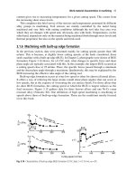
Figure 1 shows the fit of this distribution to the data of one of the texts on the basis of
Fig. 1. Rank-Frequency Distribution of L-Segments
L-segments on a log-log scale. In this case, the goodness-of-fit test yielded P(F
2
) ≈
640 Reinhard Köhler and Sven Naumann
1.0 with 92 degrees of freedom. N = 941 L-segments were found in the text forming
x
max
= 112 different patterns. Similar results were obtained for all three kinds of
segments and all texts. Various experiments with the frequency distributions show
promising differences between authors and genres. However, these differences alone
do not yet allow for a crisp discrimination.
4 Length distribution of L-segments
As a consequence of our general hypothesis, not only the segment types but also the
length of the segments should follow lawful patterns. Here, we study the distribution
of L-segment length. First, a theoretical model is set up on the basis of three plausible
assumptions:
1. There is a tendency in natural language to form compact expressions. This can be
achieved at the cost of more complex constituents on the next level. An example
is the following: The phrase "as a consequence" consists of 3 words, where the
word "consequence" has 3 syllables. The same idea can be expressed using the
shorter expression "consequently", which consists of only 1 word of 4 syllables.
Hence, more compact expressions on one level go along with more complex
expressions on the next level. Here, the consequence of the formation of longer
words is relevant. The variable K will represent this tendency.
2. There is an opposed tendency, viz. word length minimization. It is a consequence

of the same tendency of effort minimization which is responsible for the first
tendency but now considered on the word level. We will denote this requirement
by M.
3. The mean word length in a language can be considered as constant, at least for a
certain period of time. This constant will be represented by q.
According to a general approach proposed by Altmann (cf. Altmann and Köhler
(1996)) and substituting k = K −1andm = M −1, the following equation can be set
up:
P
x
=
k +x−1
m + x −1
qP
x−1
(2)
which yields the hyper-Pascal distribution (cf. Wimmer and Altmann (1999)):
P
x
=

k+x−1
x


m+x−1
x

q
x

P
0
,x = 0,1,2, (3)
with P
−1
0
=
2
F
1
(k, 1;m;q) - the hyper-geometric function - as norming constant.
Here, (3) is used in a 1-displaced form because length 0 is not defined, i.e. L-
segments consisting of 0 words are impossible. As this model is not likely to be
adequate also for F- and T-segments - the requirements concerning the basic proper-
ties frequency and polytextuality do not imply interactions between adjacent levels
- a simpler one can be set up. Due to length limitations to our contribution in this
volume we will not describe the appropriate model for these segment types but it
Quantitative Text Analysis Using L-, F- and T-Segments 641
can be said here that their length distributions can be modeled and explained by the
hyper-Poisson distribution.
Fig. 2. Theoretical and empirical distribution of L-segments in a poem
Fig. 3. Theoretical and empirical distribution of L-segments in a short story
The empirical tests on the data from the 66 texts support our hypothesis with good
and very good 2 values. Figures 2 and 3 show typical graphs of the theoretical and
empirical distributions as modeled using the hyper-Pascal distribution. Figure 2 is an
example of poetry; Figure 3 shows a narrative text. Good indicators of text genre or
authors could not yet be found on the basis of these distributions. However, only a
few of the available characteristics have been considered so far. The same is true of
the corresponding experiments with F- and T-segments.
642 Reinhard Köhler and Sven Naumann

5 TTR studies
Another hypothesis investigated in our study is the assumption that the dynamic be-
havior of the segments with respect to the increase of types in the course of the given
text, the so-called TTR, is analogous to that of words or other linguistic units. Word
TTR has the longest history; the large number of approaches presented in linguistics
is described and discussed in (Altmann (1988), p. 85-90), who gives also a theo-
retical derivation of the so-called Herdan model, the most commonly used one in
linguistics:
y = x
a
, (4)
where x represents the number of tokens, i.e. the individual position of a running
word in a text, and y the number of types, i.e. different words. a is an empirical pa-
rameter. However, this model is appropriate only in case of very large inventories,
such as the vocabulary of a language. For smaller inventories, other models must be
derived (cf. Köhler, R. and Martináková-Rendeková, Z. (1998), Köhler, R. (2003a)
and Köhler, R. (2003b)). We expect model (4) to work with segment TTR, an equa-
tion, which was derived by Altmann (1980) for the Menzerath-Altmann Law and
later in the framework of synergetic linguistics:
y = ax
b
e
cx
,c < 0. (5)
The value of a can be assumed to be equal to unity, because the first segment of a
text must be the first type, of course. Therefore, we can remove this parameter from
the model and simplify (4) as shown in (5):
y = e
−c
x

b
e
cx
= x
b
e
c(x−1)
,c < 0. (6)
Figures 4 and 5 show the excellent fits of this model to data from one of the poems
and one of the prose texts. Goodness-of-fit was determined using the determination
coefficient R
2
, which was above 0.99 in all 66 cases. The parameters b and c of the
Quantitative Text Analysis Using L-, F- and T-Segments 643
Fig. 4. L-segment TTR of a poem
Fig. 5. L-segment TTR of a short story
TTR model turned out to be quite promising characteristics of text genre and author.
They are not likely to discriminate these factors sufficiently when taken alone but
seem to carry a remarkable amount of information. Figure 6 shows the relationship
between the parameters b and c.
644 Reinhard Köhler and Sven Naumann
Fig. 6. Relationship between the values of b and c in the corpus
6 Conclusion
Our study has shown that L-, F- and T-Segments on the word level display a lawful
behavior in all aspects investigated so far and that some of the parameters, in partic-
ular those of the TTR, seem promising for text classification. Further investigations
on more languages and on more text genres will give more reliable answers to these
questions.
References
ALTMANN, G. and KÖHLER, R. (1996): "Language Forces? and Synergetic Modelling of

Language Phenomena. In: P. Schmidt [Ed.]: Glottometrika 15. Issues in General Linguis-
tic Theory and The Theory of Word Length. WVT, Trier, 62-76.
ANDERSEN, S. (2005): Word length balance in texts: Proportion constancy and word-chain-
lengths in Proust’s longest sentence. Glottometrics 11, 32-50.
BORODA, M. (1982): Häufigkeitsstrukturen musikalischer Texte. In: J. Orlov, M. Boroda, G.
Moisei and I. Nadarej
ˆ
svili [Eds.]: Sprache, Text, Kunst. Quantitative Analysen. Brock-
meyer, Bochum, 231-262.
HERDAN, G. (1966): The advanced Theory of Language as Choice and Chance. Springer,
Berlin et al., 423.
KÖHLER, R. (1999): Syntactic Structures. Properties and Interrelations. Journal of Quantita-
tive Linguistics 6, 46-57.
KÖHLER, R. (2000): A study on the informational content of sequences of syntactic units.
In: L.A. Kuz’min [Ed.]: Jazyk, glagol, predlo?enie. K 70-letiju G. G. Sil’nitskogo.
Smolensk, S. 51-61.
KÖHLER, R. and G. ALTMANN (2000): Probability Distributions of Syntactic Units and
Properties. Journal of Quantitative Linguistics 7/3, S.189-200.
KÖHLER, R. (2006b): Word length in text. A study in the syntagmatic dimension. To appear.
Quantitative Text Analysis Using L-, F- and T-Segments 645
KÖHLER, R. (2006a): The frequency distribution of the lengths of length sequences. In: J.
Genzor and M. Bucková [Eds.]: Favete linguis. Studies in honour of Victor Krupa. Slovak
Academic Press, Bratislava, 145-152.
UHLÍHOVÁ, L. (2007): Word frequency and position in sentence. To appear.
WIMMER, G. and ALTMANN, G. (1999): Thesaurus of Univariate Discrete Probability Dis-
tributions. Stamm, Essen.
Structural Differentiae of Text Types – A Quantitative
Model
Olga Pustylnikov and Alexander Mehler
Faculty of Linguistics and Literature Study,

University of Bielefeld, Germany
{Olga.Pustylnikov, Alexander.Mehler}@uni-bielefeld.de
Abstract. The categorization of natural language texts is a well established research field in
computational and quantitative linguistics (Joachims 2002). In the majority of cases, the vector
space model is used in terms of a bag of words approach. That is, lexical features are extracted
from input texts in order to train some categorization model and, thus, to attribute, for exam-
ple, authorship or topic categories. Parallel to these approaches there has been some effort in
performing text categorization not in terms of lexical, but of structural features of document
structure. More specifically, quantitative text characteristics have been computed in order to
derive a sort of structural text signature which nevertheless allows reliable text categorizations
(Kelih & Grzybek 2005; Pieper 1975). This “bag of features” approach regains attention when
it comes to categorizing websites and other document types whose structure is far away from
the simplicity of tree-like structures. Here we present a novel approach to structural classifiers
which systematically computes structural signatures of documents. In summary, we present
a text categorization algorithm which in the absence of any lexical features nevertheless per-
forms a remarkably good classification even if the classes are thematically defined.
1 Introduction
An alternative way to categorize documents apart from the well established “ bag of
words” approach is to categorize by means of structural features. This approach func-
tions in absence of any lexical information utilizing quantitative characteristics of
documents computed from the logical document structure.
1
That means that markers
like content words are completely disregarded. Features like distributions of sections,
paragraphs, sentence length etc. are considered instead.
Capturing structural properties to build a classifier assumes that given category
separations are reflected by structural differences. According to Biber (1995) we can
expect that functional differences correlate with structural and formal representa-
tions of text types. This may explain good overall results in terms of F-Measure
2

.
1
See also Mehler et al. (2006).
2
The harmonic mean of precision and recall is used here to measure the overall success of
the classification
656 Olga Pustylnikov and Alexander Mehler
However, the F-Measure gives no information about the quality of the investigated
categories. That is, no a prior knowledge about the suitability of the categories for
representing homogenous classes and for applying them in machine learning tasks is
provided. Since natural language categories e.g. in form of web documents or other
textual units arise not necessarily with a well defined structural representation avail-
able it is important to know how the classifier behaves dealing with such categories.
Here, we investigate a large number of existing categories, thematic classes or
rubrics taken from a 10 years newspaper corpus of Süddeutsche Zeitung (SZ 2004)
whereas a rubric represents a recurrent part of the newspaper like `sportst’ or `tv-
newst’. We test systematically their goodness in a structural classifier framework ask-
ing more specifically for a maximal subset of all rubrics which gives an F-Measure
above a predefined cut-off c ∈ [0, 1] (e.g. c = 0.9). We evaluate the classifier in the
way allowing to exclude possible drawbacks with respect to:
• the categorization model used (here SVM
3
and Cluster Analysis),
4
• the text representation model used (here the bag of features approach) and
• the structural homogeneity of categories used.
The first point relates to distinguishing supervised and unsupervised learning. That
is, we perform these sorts of learning although we do not systematically evaluate
them comparatively with respect to all possible parameters. Rather, we investigate
the potential of our features evaluating them with respect to both scenarios. The

representation format (vector representation) is restricted by the model used (e.g.
SVM). Thus, we concentrate on the third point and apply an iterative categorization
procedure (ICP)
5
to explore the structural suitability of categories. In summary, our
experiments have twofold goals:
1. to study given categories using the ICP in order to filter out structurally incon-
sistent types and
2. to make judgements about the structural classifier’s behavior dealing with cate-
gories of different size and quality levels.
2 Category selection
The 10 years corpus of the SZ used in the present study contains 95 different rubrics.
The frequency distribution of these rubrics shows an enormous inequality for the
whole set (See Figure 1). In order to minimize the calculation effort we reduce the
initial set of 95 rubrics to a smaller subset according to the following criteria.
1. First, we compute the mean z and the standard deviation V for the whole set.
3
Support Vector Machines.
4
Supervised vs. unsupervised respectively.
5
See sec. 4.
Structural Differentiae of Text Types – A Quantitative Model 657
0 10 20 30 40 50 60 70 80 90 100
0
2000
4000
6000
8000
10000

12000
Categories
Articles
95 Rubrics of SZ
Fig. 1. Categories/Articles-Distribution of 95 Rubrics of SZ.
2. Second, we pick out all rubrics R with the cardinality |R| (the number of exam-
ples within the corpus) ranging between the interval:
z −V/2 < |R| < z +V/2
This selection method allows to specify a window around the mean value of all doc-
uments leaving out the unusual cases.
6
Thus, the resulting subset of 68 categories is
selected.
3 The evaluation procedure
The data representation format for the subset of rubrics uses a vector representation
(bag of features approach) where each document is represented by a feature vector.
7
The vectors are calculated as structural signatures of the underlying documents. To
avoid drawbacks (See Sec. 1) caused by the evaluation method in use, we compare
three different categorization scenarios:
1. Supervised scenario by means of SVM-light
8
,
2. Unsupervised scenario in terms of Cluster Analysis and
3. Finally, a baseline experiment based on random clustering.
6
The method is taken from Bock (1974). Rieger (1989) uses it to identify above-average
agglomeration steps in the clustering framework. Gleim et al. (2007) successfully applied
the method to develop quality filters for wiki articles.
7

See Mehler et al. (2007) for a formalization of this approach.
8
Joachims (2002).
658 Olga Pustylnikov and Alexander Mehler
Consider an input corpus K and a set of categories C with the number of categories
|C| = n. Then we proceed as follows to evaluate our various learning scenarios:
• For the supervised case we train a binary classifier by treating the negative ex-
amples of a category C
i
∈ C as K \[C
i
] and the positive examples as a subset
[C
i
] ⊆ K. The subsets C
i
are in this experiment pairwise disjunct and we define
L = {[C
i
]|C
i
∈ C} as a partition of positive and negative examples of C
i
.
Classification results are obtained in terms of precision and recall. We calculate
the F-score for a class C
i
in the following way:
F
i

=
2
1
recall
i
+
1
precision
i
In the next step we compute the weighted mean for all categories of the partition
L in order to judge about the overall separability of given text types using the
F-Measure:
F-Measure(L)=
n

i
|C
i
|
|K|
F
i
• In the case of unsupervised experiments we approach as follows: The unsu-
pervised procedure evaluates different variants of Cluster Analysis (hierarchi-
cal, k-means) trying out several linkage possibilities (complete, single, average,
weighted) in order to achieve the best performance. Similar to the supervised
case best clustering results are presented in terms of F-Measure values.
• Finally, the random baseline is calculated by preserving the original category
sizes and by mapping articles randomly to them. Results of random clustering
help to check the success of both learning scenarios. Thus, clusterings close to

the random baseline indicate either a failure of the cluster algorithm or that the
separability of the text types can’t be well separated by structure.
In summary, we check the performance of structural signatures within two learning
scenarios – supervised and unsupervised – and compare the results with the random
clustering baseline. Next Section describes the incremental categorization procedure
(ICP) to investigate the structural homogeneity of categories.
4 Exploring the structural homogeneity of text types by means of
the Iterative Categorisation Procedure (ICP)
In this Section we return to the question mentioned at the beginning. Given a cut-
off c ∈ [0,1] (e.g. c = 0.9) we ask for the maximal subset of rubrics allowing to
achieve an F-Measure value F > c. Decreasing the cut-off c successively we get a
rank ordering of rubrics ranging from the best contributors to the worst ones. The
ICP allows to determine a result set of maximal size n with the maximal internal
homogeneity compared to all candidate sets in question. Starting with a given set of
input categories to be learned we proceed as follows:
Structural Differentiae of Text Types – A Quantitative Model 659
1. Start: Select a seed category C ∈ A and set A
1
= {C}. The rank r of C equals
r(C)=1. Now repeat:
2. Iteration (i > 1): Let B = A\A
i−1
. Select the category C ∈B which when added
to A
i−1
maximizes the F-Measure value among all candidate extensions of A
i−1
by means of single categories of B.SetA
i
= A

i−1
∪{C} and r(C)=i.
3. Break off: The iteration algorithm terminates if either
i) A \A
i
=

 or
ii) the F-Measure value of A
i
is smaller than a predefined cut-off or
iii) the F-Measure value of A
i
is smaller than the one of the operative baseline.
If none of these stop conditions holds repeat step (2).
The kind of ranking described here is more informative than the F-Measure value
alone. That is, the F-Measure gives global information about the overall separabil-
ity of categories. The ICP in contrast, provides additional local information about
the weights of single categories with respect to the overall performance. This in-
formation allows to check the suitability of single categories to serve as structural
prototypes. Knowledge about the homogeneity of each category provides a deeper
insight into the possibilities of our approach.
In the next Section the rankings of the ICP applied to supervised and unsuper-
vised learning and compared with the random clustering baseline are presented. In
order to exclude a dependence of the structural approach on one of the learning me-
thods, we also apply the best-of-unsupervised-ranking to the supervised scenario and
compare the outcomes. That means, we use exactly the same range having performed
best in the unsupervised experiment for SVM learning.
5 Results
Table 1 gives an overview about the categories used. From the total number of 95

rubrics 68 were selected using the selection method described in Section 2, 55 were
considered in unsupervised, 16 in supervised experiments. The common subset used
in both cases consists of 14 categories.
The Y-axis of Figure 2 represents the F-Measure values and the X-axis the rank
order of categories iteratively added to the seed set. The supervised scenario (upper
curve) performs best ranging around the value of 1.0. The values of the unsupervised
case decrease more rapidly (the third curve from above). The unsupervised best-
of-ranking categorized with the supervised method (second curve from above) lies
between the best results of the two methods. The lower curve represents the results
of random clustering.
6 Discussion
According to Figure 2 we can see, that all F-Measure results lie high above the
baseline of random clustering. All the subsets are well separated by their document
660 Olga Pustylnikov and Alexander Mehler
Table 1. Corpus Formation (by Categories).
Category Set Number
Total 95
Selected Initial Set 68
Unsupervised 55
Supervised 16
Unsupervised ∩ Supervised 14
Fig. 2. The F-Measure Results of All Experiments
structure which indicates a potential of structure-based categorizations. The point
here was to observe the decrease of the F-Measure value while adding new cate-
gories.
The supervised method shows the best results remaining stable with a grow-
ing number of additional categories. The unsupervised method shows a more rapid
decrease but is less time consuming. Cluster Analysis succeeds to rank 55 rubrics
whereas SVM-light ranks only 16 within the same time span.
In order to compare the performance of both methods (supervised vs. unsuper-

vised) more precisely we ran the supervised categorization based on the best-off-
ranking of the unsupervised case. The resulting curve remains longer stable than the
unsupervised one. Since the order and the features of categories are equal, the re-
sulting difference indicates an overall better accuracy of SVM compared to Cluster
Analysis.
One assumption for the success of the structural classifier was that the perfor-
mance may depend on the article size, that is, on the representativeness of a category.
To account for this, we compared the category size of the best-off-rankings of both
Structural Differentiae of Text Types – A Quantitative Model 661
Fig. 3. Categories/Articles-Distribution of Sets used in Supervised/Unsupervised Experi-
ments.
experiments. Figure 3 shows a high variability in size, which indicates that the size
factor does not influence the classifier.
7 Conclusion
In this paper we presented experiments which shed light on the possibilities of a
classifier operating with structural signatures of text types. More specifically, we in-
vestigated the ability of the classifier to deal with a large number of natural language
categories of different size and quality. The best-off-rankings showed that different
evaluation methods (supervised/unsupervised) prefer different combinations of cat-
egories to achieve the best separation. Furthermore, we could see that the overall
difference in performance of two methods depends rather on the method used than
on the combination of categories.
Another interesting finding is that the structural classifier seems not to depend on
category size allowing a good categorization of small, less representative categories.
That fact motivates to use logical document (or any other kind of) structure for ma-
chine learning tasks and to extend the framework to more demanding tasks, when it
comes to deal with, e.g., web documents.
662 Olga Pustylnikov and Alexander Mehler
References
ALTMANN, G. (1988): Wiederholungen in Texten. Brockmeyer, Bochum.

BIBER, D. (1995): Dimensions of Register Variation: A Cross-Linguistic Comparison. Uni-
versity Press, Cambridge.
BOCK, H.H. (1974): Automatische Klassifikation. Theoretische und praktische Methoden
zur Gruppierung und Strukturierung von Daten (Cluster-Analyse). Vandenhoeck &
Ruprecht, Göttingen.
GLEIM, R.; MEHLER, A.; DEHMER, M.; PUSTYLNIKOV, O. (2007): Isles Through the
Category Forest — Utilising the Wikipedia Category System for Corpus Building in Ma-
chine Learning. In: WEBIST ’07, WIA(2). Barcelona, Spain, 142-149.
JOACHIMS, T. (2002): Learning to classify text using support vector machines.Kluwer,
Boston/Dordrecht/London.
KELIH, E.; GRZYBEK, P. (2005): Satzlänge: Definitionen, Häufigkeiten, Modelle (Am
Beispiel slowenischer Prosatexte). In: LDV-Forum 20(2), 31-51.
MEHLER, A.; GEIBEL, P.; GLEIM, R.; HEROLD, S.; JAIN, B.; PUSTYLNIKOV, O. (2006):
Much Ado About Text Content. Learning Text Types Solely by Structural Differentiae.
In: OTT’06.
MEHLER, A.; GEIBEL, P.; PUSTYLNIKOV, O.; HEROLD, S. (2007): Structural Classifiers
of Text Types. To appear in: LDV Forum.
PIEPER, U. (1975): Differenzierung von Texten nach Numerischen Kriterien. In: Folia Lin-
guistica VII, 61-113.
RIEGER, B. (1989): Unscharfe Semantik: Die empirische Analyse, quantitative Beschreibung,
formale Repräsentation und prozedurale Modellierung vager Wortbedeutungen in Texten.
Peter Lang, Frankfurt a. M.
SÜDDEUTSCHER VERLAG (2004). Süddeutsche Zeitung 1994-2003. 10 Jahre auf DVD.
München.
The Distribution of Data in Word Lists and
its Impact on the Subgrouping of Languages
Hans J. Holm
Hannover, Germany

Abstract. This work reveals the reason for the bias in the separation levels computed for

natural languages with only a small amount of residues; as opposed to stochastically normal
distributed test cases like those presented in Holm (2007a). It is shown how these biased
data can be correctly projected to true separation levels. The result is a partly new chain of
separation for the main Indo-European branches that fits well to the grammatical facts, as well
as to their geographical distribution. In particular it strongly demonstrates that the Anatolian
languages did not part as first ones and thereby refutes the Indo-Hittite hypothesis.
1 General situation
Traditional historical linguists use a priori to look upon quantitative methods with
suspicion, because they argue that only those agreements can decide the question,
which are supposed to stem exclusively from their direct ancestor, the so-called
‘common innovations’, or synapomorphies, in biological terminology (Hennig 1966).
However, this seemingly perfect concept has in over a hundred years of research
brought about anything but agreement on even a minimum of groupings (e.g. those
in Hamp 2005). There is no grouping, which is not debated in one or more ways.
‘Lumpers’ and ‘splitters’ are at work, as with nearly all proposed language families.
Quantitative attempts (cf. Holm (2005), to be updated (2007b), for an overview)
have not proved to be superior: First, all regard such trivial results like distinguish-
ing e.g. Greek from Germanic as a proof; secondly, many of them are fixated on a
mechanistic rate (or “clock") assumption for linguistic changes (what is not our fo-
cus here); and worst, mathematicians, biologists, and even some linguists retreat to
the too loose view that the amount of agreements is a direct measure of relatedness.
Elsewhere I have demonstrated that this assumption is erroneous because these re-
searchers overlook the dependence of this surface phenomenon from at least three
stochastic parameters, the “proportionality trap" (cf. Holm (2003); Swofford et al.
(1996:487)).
630 Hans J. Holm
2 Special situation
2.1 Recapitulation: What is the proportionality trap?
Definition: If a “mother" language splits into (two) daughter languages, these are
“genealogically related". At the point of split, or era of separation, both start with the

full amount of inherited features. However, they will soon begin to differentiate by
loss or replacement of these original features. These individual replacements occur
• independently (!) from each other,
• by new irregular socio-psychological impacts in history. They are therefore non-
deterministic in that the next state of the environment is partially but not fully
determined by the previous state. Least, they are
• irreversible, because, when a feature is changed, it will normally never reappear.
Fig. 1. Different agreements, same relationship(!)
Because of these properties we have to regard linguistic change mathematically
as a stochastic process by draws without replacement. Any statistician will immedi-
ately recognize this as the hypergeometric distribution. In word lists, we in fact have
all four parameters (cf. Fig. 1) needed as follows:
• The amount of inherited features k
i
and k
j
(or residues, cognates, symplesiomor-
phies) regarded as preserved from the common ancestor of any two languages L
i
and L
j
;
• the amount of shared agreements ‘a
i, j
’ between them;
• the amount N of their common features at the time of separation (the universe),
not visible in the surface structure of the data. Exactly this invisible universe N
are we seeking for, because it represents the underlying structure, the amount
of features, which must have been present in both languages at the era of their
Distribution of Data in Word Lists 631

separation in the past. And again any mathematician has the solution: This “sep-
aration level" N for each pair of branches can be estimated by the 2
nd
momentum
of the hypergeometric, the maximum likelihood estimator, transposed to
ˆ
N = k
i
×k
j

a
i,j
Since changes can only lower the number of common features, a higher separation
level must lie earlier in time, and thus we obtain a ranked chain of separation in a
family of languages.
2.2 Applications up to now
The first one to propose and apply this method was the British mathematician D.G.
Kendall (1950) with the Indo-European data of Walde/Pokorny (1926-32). It has
then independently been extensively applied to the data of the improved dictionary
of Pokorny (1959) by Holm (2000, passim). The results seemed to be convincing,
in particular for the North-Western group, and also for the relation of Greek and the
Indo-Iranian group. The late separations of Albanian, Armenian, and Hittite could
well have been founded in their central position and therefore did not appear suspi-
cious.
Only when in a further application to Mixe-Zoquean data by Cysouw et al. (2006)
a resembling observation occurred that only languages with few known residues ap-
peared to separate late, a systematic bias could be suspected. Cysouw et al. discarded
the SLR-method, because their results partly contradicted the subgrouping of Mixe-
Zoquean as inferred by traditional methods of two historical linguists (which in fact

did not completely agree with each other). In a presentation Cysouw (2004) sus-
pected that the “unbalanced amount of available data distorts the estimates", and
“Error 1: they are grouped together, because of many shared retentions.” However,
this only demonstrates that the basics explained above are not correctly understood,
since the hypergeometric does just not rest on one parameter alone.
In this study we will use the most modern and acknowledged Indo-European
data base, the “Lexikon der indogermanischen Verben" (Rix et al. (2002), henceforth
LIV-2. I am very obliged to the authors for sending me the digitalized version, which
in fact only enabled me to quantify the contents in acceptable time. The reasons for
this tremendous undertaking were:
• The commonplace (though seldom mentioned) in linguistics that verbs are much
lesser borrowed than nouns, what is not taken into account by any quantitative
work up to now.
• The more trustworthy combined work of a team at an established department of
Indo-European under the supervision of a professional historical linguist should
guarantee a very high standard, moreover in this second edition.
• Compared with the in many parts outdated Pokorny, we have now much better
knowledge of the Anatolian and Tocharian languages.
632 Hans J. Holm
Fig. 2. Unwanted dependence N from k in LIV-2 list
3 The bias
3.1 Unwanted dependence
Nevertheless, these much better data, not suspicious of poor knowledge, displayed
the same bias as the other ones, as demonstrated in Fig. 2, which presents the corre-
lation between the residues ‘k’ and the corresponding ‘
ˆ
N’s in falling order. Thus we
have a problem. The reason for this bias, opposite to Cysouw et al., could not lie in
a poor knowledge of the data, nor could it lie in the algorithm, as I have additionally
tested in hundreds of random cases, some of which published in Holm (2007a). Con-

sequently, the reason had to be found in the word lists alone, the properties of which
we will have to inspect now with closer scrutiny:
3.2 Revisiting the properties of word lists
The effects of scatter on the subgrouping problem as well as its handling has been
intensively investigated by Holm (2007a). This study as well as textbooks suggest
that the sum of residues ‘k’ should exceed at least 90 % of the universe ‘N’, and
a single ‘k’ must not fall below 20 %. However, since the LIV-2 database is big
enough to guarantee a low scatter, there must be something else, overlooked up to
now. A first hint has already been given by D.G. Kendall (1950:41), who noticed that
“One must, however, assume that along a given segment of a given line of descent
the chance of survival is the same for every root exposed to risk, and one must also
assume that the several roots are exposed to risk independently". The latter condition
Distribution of Data in Word Lists 633
is the easier part, since linguists would agree that changes in the lexicon or grammar
occur independently of each other. (The so-called push-and-pull chains are mainly a
phonetic symptom and of lesser interest here). The real problem is the first condition,
since the chance of survival is not at all the same for any feature, and every word has
its own history. For our purpose, we must not necessarily deal with the reasons for
these changes in detail. Could the reason for the observed bias perhaps be found in a
distribution that contradicts the conditions of the hypergeometric, and perhaps other
quantitative approaches, too?
3.3 The distribution in word lists
For that purpose, the 1195 reconstructed verbal roots of the LIV-2 are entered as
“characters” into a spreadsheet, while the columns contain the 12 branches of Indo-
European. We let then sum up the cross totals into a new column, containing now
the frequency for every row. After sorting to these, we get twelve different blocks
or slices, one for each frequency. By counting out every language per slice, we get
12 matrices, of which we enter the arithmetic means into the final table. Let us now
have a closer look at the plot of this as Fig. 3.
Fig. 3. All frequencies of the LIV-2 data

634 Hans J. Holm
3.4 Detecting the reason
Immediately we observe to the right hand the few verbs which occur in many lan-
guages, growing up to the left with the many verbs occurring in fewer languages,
breaking down to the special case of verbs occurring in one language only. To find
out the reason of the false correlation between these curves and the bias with the
smaller represented languages, we must first identify the connections with our for-
mula:
ˆ
N depends on the product of the residues ‘k’ of any language, as represented
here as the area below their curve. This product is then divided by their agreements
‘a’, which are naturally represented by the frequencies (bottom line). And here - not
easily to detect - lies the key: The more to the right hand, the higher the agreements
per residue. Further: The smaller the sum of residues of a branch (area below its
curve), the higher is the proportion of agreements, ending in a false lower separation
level. So far we have located the problem. But we are still far from a solution.
4 Solution and operationalization
Since the bias will turn up every time one employs the total of the data, we must
compute every slice separately, thereby using only data with the same chance of
being replaced. Restrictions in printing space do not allow to address the different
options of implementations. In any case, it is extremely useful to pre-order the nu-
merical outcome according to the presumptive next neighbor of every branch by the
historical-bundling (“Bx”) method, explained in Holm (2000:84-5, or 2005:640). Fi-
nally, the matrix allows us to reconstruct the tree. To avoid the attractions, deletions,
and other new bias resulting from traditional clustering methods, it is methodologi-
cally advisable to proceed on a broad front. That means, first to combine every branch
with its next neighbor (if their is one), and only then proceed this way uphill, find-
ing the next node by the arithmetic mean of the cross fields. This helps very well to
rule out the unavoidable scatter. Additionally, the above-mentioned Bx-values are in
particular helpful to “flatten" the graph, which naturally is only ordered in the one di-

rection of descent, but might represent different clusters or circles in real geography,
what is not displayable in such two-dimensional graph.
5 Discussion
Though we have ruled out the bias in the distributions of word lists, there could
well be more bias hidden in the data: Extremely different cultural backgrounds be-
tween compared branches would lead to fewer agreements and thus false earlier split.
An example are the Baltic languages in a cultural environment of hunter- and gath-
erer communities vs. the Anatolian languages in an environment of advanced civ-
ilizations. Secondly, there may be left differences in the reliability of the research
itself. Third, it is well-known that the relative position of the branches give raise to
more innovations in the center vs. more conservative behavior in peripheral positions
(“Saumlage”).
Distribution of Data in Word Lists 635
Fig. 4. New SLRD-based tree of the main IE branches
6 Conclusions
Linguistically, this study clearly refutes an early split of/from Anatolian and thereby
the “Indo-Hittite” Hypothesis. Methodologically, the former “Separation-Level Re-
covery method” is updated to one accounting for the Distribution (SLRD). The in-
sights gained should prevent everybody from trusting methods not regarding the hy-
pergeometric behavior of language change, as well as the distribution in word lists.
People must not be dazzled by apparently good results, which regularly appear, due
alone to very strong signals in the data, or simply by chance.
References
CYSOUW, M. (2004): email.eva.mpg.de/ cysouw/pdf/cysouwWIP.pdf
CYSOUW, M., WICHMANN, S. and KAMHOLZ, D. (2006): A critique of the separation
base method for genealogical subgrouping, with data from Mixe-Zoquean. Journal of
Quantitative Linguistics, 13(2-3), 225–264.
EMBLETON, S.M. (1986): Statistics in historical linguistics [Quantitative Linguistics 30].
Brockmeyer, Bochum.
GRZYBEK, P., and R. KÖHLER (Eds). (2007): Exact Methods in the Study of Language and

Text [Quantitative Linguistics 62]. De Gruyter Berlin.
HAMP, E.P. (1998): “Whose were the Tocharians? Linguistic subgrouping and Diagnostic
Idiosyncrasy” The Bronze Age and Early Iron Age Peoples of Eastern Central Asia. Vol.
1:307-46. Edited by Victor H. Mair. Washington DC: Institute for the Study of Man.
636 Hans J. Holm
HOLM, H.J. (2000): Genealogy of the Main Indo-European Branches Applying the Separation
Base Method. Journal of Quantitative Linguistics, 7-2, 73–95.
HOLM, H.J. (2003): The proportionality trap; or: What is wrong with lexicostatistics? In-
dogermanische Forschungen 108, 38–46.
HOLM, H.J. (2007a): Requirements and Limits of the Separation Level Recovery Method in
Language Subgrouping. In: GRZYBEK, P. and KÖHLER, R. (Eds), Viribus Quantitatis.
Exact Methods in the Study of Language and Text. Festschrift Gabriel Altmann zum 75.
Geburtstag. Quantitative Linguistics 62. De Gruyter, Berlin.
HOLM, H.J. (to appear 2007b): The new Arboretum of Indo-European “Trees”. Journal of
Quantitative Linguistics 14-2.
KENDALL, D.G. (1950): Discussion following Ross, A.S.C., Philological Probability Prob-
lems. Journal of the Royal Statistical Society, Ser. B 12, p. 49f.
POKORNY, J. (1959): Indogermanisches etymologisches Wörterbuch. Francke, Bern.
RIX, H., KÜMMEL, M., ZEHNDER, Th., LIPP, R. and SCHIRMER, B. (2001): Lexikon
der indogermanischen Verben. Die Wurzeln und ihre Primärstammbildungen.2.Aufl.
Reichert, Wiesbaden.
SWOFFORD, D.L., OLSEN, G.J., Waddell, P.J., and HILLIS, D.M. (1996): “Phylogenetic
Inference”. In: HILLIS, D.M., M. CRAIG, and B.K. MABLE (Eds). Molecular System-
atics, Second Edition. Sinauer Associates, Sunderland MA, Chapter 11.
WALDE, A., and J. Pokorny (Ed). (1926-1932): Vergleichendes Wörterbuch der indogerman-
ischen Sprachen. de Gruyter, Berlin.
A New Interval Data Distance Based on the
Wasserstein Metric
Rosanna Verde and Antonio Irpino
Dipartimento di Studi Europei e Mediterranei

Seconda Universitá degli Studi di Napoli - Caserta (CE), Italy
{rosanna.verde, antonio.irpino}@unina2.it
Abstract. Interval data allow statistical units to be described by means of interval values,
whereas their representation by single values appears to be too reductive or inconsistent, that
is, unable to keep the uncertainty usually inherent to the observed data. In the present paper,
we present a novel distance for interval data based on the Wasserstein distance between dis-
tributions. We show its interesting properties within the context of clustering techniques. We
compare the obtained results using the dynamic clustering algorithm, taking into consideration
different distance measures in order to justify the novelty of our proposal.
1
1 Introduction
The representation of data by means of intervals of values is becoming more and
more frequent in different fields of application. In general, an interval description
depends on the uncertainty that affects the observed values of a phenomenon. The
uncertainty can be considered as the inability to obtain true values depending on ig-
norance of the model that regulates the phenomenon. This uncertainty can be of three
types: randomness, vagueness or imprecision (Coppi et al., 2006). Randomness is
present when it is possible to hypothesize a probability distribution of the outcomes
of an experiment, or when the observation is affected by an error component that is
modeled as a random variable (i.e., white noise in a Gaussian distribution). Vague-
ness is related to an unclear fact or whether the concept even applies. Imprecision is
related to the difficulty of accurately measuring a phenomenon. While randomness
is strictly related to a probabilistic approach, vagueness and imprecision have been
widely treated using fuzzy set theory, as well as the interval algebra approach. Prob-
abilistic, fuzzy and interval algebra sometimes overlap in treating interval data. In
the literature, interval algebra and fuzzy theory are treated very closely, especially in
defining dissimilarity measures for the comparison of values affected by uncertainty
expressed by intervals.
Interval data have even been studied in Symbolic Data Analysis (SDA) (Bock and
Diday (2000)), a new domain related to multivariate analysis, pattern recognition and

1
The present paper has been supported by the LC
3
Italian research project.
706 Rosanna Verde and Antonio Irpino
artificial intelligence. In this framework, in order to take into account the variability
and/or the uncertainty inherent to the data, the description of a single unit can assume
multiple values (bounded sets of real values, multi-categories, weight distributions),
where intervals are a particular case. In SDA, several dissimilarity measures have
been proposed. Chavent and Lechevallier (2002) and Chavent et al. (2006) proposed
Hausdorff L
1
distances, while De Carvalho et al. (2006) proposed L
q
distances and
De Souza et al. (2004) an adaptive L
2
version. It is worth noting that these measures
are based essentially on the boundary values of the compared intervals. These dis-
tances have been mainly proposed as criterion functions in clustering algorithms to
partition a set of interval data where a cluster structure can be assumed.
In the present paper, we present some dissimilarity (or distance) functions, pro-
posed in fuzzy, symbolic data analysis and probabilistic contexts to compare intervals
of real values. Finally, we introduce a new metric based on the Wasserstein distance
that respects all the classical properties of a distance and, being based on the quantile
functions associated with the interval distributions, seems particularly able to keep
the whole information contained in the intervals and not only on the bounds.
The structure of the paper is as follows: in Section 2, some families of distances
for interval data, arising by different contexts, are shown. In Section 3, the new dis-
tance, based on a probabilistic metric, as the L

2
version of the Monge-Kantorovich-
Wasserstein-Gini metric between quantile functions (usually known as Wasserstein
metric), is introduced. In Section 4, the performances of the proposed distance are
compared in a clustering process of a set of interval data. The obtained partition is
compared to an expert one. Therefore, performing the clustering by Adaptive L
2
as
well as Hausdorff L
1
distance, the proposed distance provides again the best results
in terms of the Correct Rand Index. Section 5 closes the paper with some remarks
and perspectives.
2 A brief survey of the existing distances
According to Symbolic Data Analysis, an interval variable X is a correspondence
between a set E of units and a set of closed intervals [a,b], where a ≤ b and a,b ∈R.
Without losing in generality, the notation is quite the same for the interval algebra
approach.
Let A and B be two intervals described, respectively, by [a,b] and [u,v]. d(A,B)
can be considered as a distance if the main properties that define a distance are
achieved: d(A,A)=0 (reflexivity), d(A,B)=d(B,A) (symmetry) and d(A,B) ≤
d(A,C)+d(C,B) (triangular inequality).
Hereinafter, we present some of the most used distances for interval data. The
main properties of such measures are even underlined.
Tran and Duckstein distance between intervals. Some of these distances have been
developed within the framework of the fuzzy approach. One of these is the distance
defined by Tran and Duckstein (2002) that has the following formulation: