578 Berenike Loos and Chris Biemann
As an application, we operate on automatic address extraction from web pages for
the tourist domain.
1.1 Motivation: Address extraction from the web
In an open-domain spoken dialog system, the automatic learning of ontological con-
cepts and corresponding relations between them is essential as a complete manual
modeling of them is neither practicable nor feasible due to the continuously chang-
ing denotation of real world objects. Therefore, the emergence of new entities in the
world entails the necessity of a method to deal with those entities in a spoken dialog
system as described in Loos (2006).
As a use case to this challenging problem we imagine a user asking the dialog
system for a newly established restaurant in a city, e.g. (“How do I get to the Auer-
stein"). So far, the system does not have information about the object and needs the
help of an incremental learning component to be able to give the demanded answer
to the user. A classification as well as any other information for the word “Auerstein"
are hitherto not modeled in the knowledge base and can be obtained by text mining
methods as described in Faulhaber et al. (2006). As soon as the object is classified
and located in the system’s domain ontology, it can be concluded that it is a building
and that all buildings have addresses. At this stage the herein described work comes
into play, which deals with the extraction of addresses in unstructured text. With a
web service (as part of the dialog system’s infrastructure) the newly found address
for the demanded object can be used for a route instruction.
Even though structured and semi-structured texts such as online directories can
be harvested as well, they often do not contain addresses of new places and do,
therefore, not cover all addresses needed. However, a search in such directories can
be used in combination with the method described herein, which can be used as a
fallback solution.
1.2 Unsupervised learning supporting supervised methods
Current research in supervised approaches to NLP often tries to reduce the amount
of human effort required for collecting labeled examples by defining methodologies
and algorithms that make a better use of the training set provided. Another promis-

ing direction to tackle this problem is to empower standard learning algorithms by
the addition of unlabeled data together with labeled texts. In the machine learning
literature, this learning scheme has been called semi-supervised learning (Sarkar and
Haffari, 2006). The underlying idea behind our approach is that syntactic and seman-
tic similarity of words is an inherent property of corpora, and that it can be exploited
to help a supervised classifier to build a better categorization hypothesis, even if the
amount of labeled training data provided for learning is very low. We emphasize
that every contribution to widening the acquisition bottleneck is useful, as long as
its application does not cause more extra work than the contribution is worth. Here,
we provide a methodology to plug an unsupervised tagger into an address extraction
system and measure its contribution.
Supporting Web-based Address Extraction with Unsupervised Tagging 579
2 Data preparation
In our semi-supervised setting, we require two different data sets: a small, manually
annotated dataset used for training our supervised component, and a large, unanno-
tated dataset for training the unsupervised part of the system. This section describes
how both datasets were obtained. For both datasets we used the results of Google
queries for places as restaurants, cinemas, shops etc. To obtain the annotated data
set, 400 of the resulting Google pages for the addresses of the corresponding named
entities were annotated manually with the labels:
street
,
house
,
zip
and
city
, all
other tokens received the label
O

.
As the unsupervised learning method is in need of large amounts of data, we used
a list with about 20,000 Google queries each returning about 10 pages to obtain an
appropriate amount of plain text. After filtering the resulting 700 MB raw data for
German language and applying cleaning procedures as described in (Quasthoff et al.,
2006) we ended up with about 160 MB totaling 22.7 million tokens. This corpus was
used for training the unsupervised tagger.
3 Unsupervised tagging
3.1 Approach
Unlike in standard (supervised) tagging, the unsupervised variant relies neither on a
set of predefined categories nor on any labeled text. As a tagger is not an application
of its own right, but serves as a pre-processing step for systems building upon it, the
names and the number of syntactic categories is very often not important.
The system presented in Biemann (2006a) uses Chinese Whispers clustering
(Biemann, 2006b) on graphs constructed by distributional similarity to induce a lex-
icon of supposedly non-ambiguous words with respect to part of speech (PoS) by
selecting only safe bets and excluding questionable cases from the category build-
ing process. In this implementation two clusterings are combined, one for high and
medium frequency words, the other collecting medium and low frequency words.
High and medium frequency words are clustered by similarity of their stop word
context feature vectors: a graph is built, including only words that are endpoints of
high similar pairs. Clustering this graph of typically 5,000 vertices results in several
hundred clusters, which are subsequently used as PoS categories. To extend the lex-
icon, words of medium and low frequency are clustered using a graph that encodes
similarity of significant neighbor co-occurrences (as defined in Dunning, 1993). Both
clusterings are mapped by overlapping elements into a lexicon that provides PoS in-
formation for some 50,000 words.
For obtaining a clustering on datasets of this size, an effective algorithm like Chi-
nese Whispers is crucial. Increased lexicon size is the main difference between this
and other approaches (e.g. (Schütze, 1995), (Freitag , 2004)), that typically operate

with 5,000 words. Using the lexicon, a trigram tagger with a morphological exten-
sion is trained, which can be used to assign tags to all tokens in a text. The tag sets
580 Berenike Loos and Chris Biemann
obtained with this method are usually more fine-grained than standard tag sets and
reflect syntactic as well as semantic similarity. In Biemann (2006a), the tagger output
was directly evaluated against supervised taggers for English, German and Finnish
via information-theoretic measures. While it is possible to relatively compare the per-
formance of different components of a system or different systems along this scale,
it does only give a poor impression on the utility of the unsupervised tagger’s output.
Therefore, an application-based evaluation is undertaken here.
3.2 Resulting tagset
As described in Section 2, we had a relatively small corpus in comparison to previ-
ous work with the same tagger, that typically operates on about 50 million tokens.
Nonetheless, the domain specifity of the corpus leads to an appropriate tagging,
which can be seen in the following examples from the resulting tag set (numbers
in brackets give the words in the lexicon per tag):
1. Nouns: Verhandlungen, Schritt, Organisation, Lesungen, Sicherung, (800)
2. Verbs: habe, lernt, wohnte, schien, hat, reicht, suchte (191)
3. Adjectives: französischen, künstlerischen, religiösen (142)
4. locations: Potsdam, Passau, Innsbruck, Ludwigsburg, Jena (320)
5. street names: Bismarckstr, Leonrodstr, Schillerstr, Ungererstr (150)
On the one hand, big clusters are formed that contain syntactic tags as shown
for the example tags 1 to 3. Items 4 and 5 show that not only syntactic tags are
created by the clustering process, but also domain specific tags, which are useful for
an address extraction. Note that the actual tagger is capable of tagging all words, not
only words in the lexicon – the number of words in the lexicon are merely the number
of types used for training. We emphasize that the comparatively small training corpus
(usually, 50M–500M tokens are employed) leaves room for improvements, as more
training text showed to have a positive impact on tagging quality in previous studies.
4 Experiments and evaluation

This section describes the supervised system, the evaluation methodology and the
results we obtained in a comparative evaluation of either providing or not providing
the unsupervised tags.
4.1 Conditional random field tagger
We perceived address extraction as a tagging task: labels indicating
city
,
street
,
house
number,
zip
code or other (
O
) from the training set are learned and applied
to unseen examples. Note that this is not comparable to a standard task like Named
Entity Recognition (cf. Roth and van den Bosch, 2002), since we are only interested
in labeling the address of the target location, and not other addresses that might be
Supporting Web-based Address Extraction with Unsupervised Tagging 581
contained in the same document. Rather, this is an instance of Information Extraction
(see Grishman, 1997). For performing the task, we train the MALLET tagger (Mc-
Callum, 2002), which is based on Conditional Random Fields (CRFs, see Lafferty
et al. 2001). CRFs define a conditional probability distribution over label sequences
given a particular observation sequence. CRFs have been proven to have equal or
superior performance at tagging tasks as compared to other systems like Hidden
Markov Models or the Maximum Entropy Framework. The flexibility of CRFs to in-
clude arbitrary, non-independent features allows us to supply unsupervised tags or no
tags to the system without changing the overall architecture. The tagger can operate
on a different set of features ranging over different distances. The following features
per instance are made available to the CRF:

• word itself
• relative position to target name
• unsupervised tag
We experimented with different orders as well as with different time shifts.
CRF order
The order of the CRF defines how many preceding labels are used for the determi-
nation of the current label. An order of 1 means that only the previous label is used,
order 2 allows for the usage of two previous labels etc. As higher orders mean more
information, which is in turn supported by fewer training examples, an optimum at
some small order can be expected.
Time shifting
Time shifting is an operation that allows the CRF to use not only the features for
the current position, but also features from surrounding positions. This is reached
by copying the features from surrounding positions, indicating what relative position
they were copied from. As with orders, an optimum can be expected for some small
range of time shifting, exhibiting the same information/sparseness trade-off. For il-
lustration, the following listing shows an original training instance with time shift 0,
as well as the same instance with time shifts -2, -1, 0, 1, 2, for the scenario with un-
supervised tags. Note that relative positions are not copied in time-shifting because
of redundancy. The following items show these shifts:
• shift 0:
– Extrablatt 0 T115
O
– 531T215
house
– Hauptstr 2 T64
street
– Heidelberg 3 T15
city
– 69117 4 T215

zip
• shift 1:
– 1 -1:Extrablatt -1:T115 0:53 0:T215 1:Hauptstr 1:T64
house
582 Berenike Loos and Chris Biemann
– 2 -1:53 -1:T215 0:Hauptstr 0:T64 1:Heidelberg 1:T15
street
• shift 2:
– 1 -2:Cafe -2:T10 -1:Extrablatt -1:T115 0:53 0:T215 1:Hauptstr 1:T64 2:Heidelberg
2:T15
house
– 2 -2:Extrablatt -2:T115 -1:53 -1:T215 0:Hauptstr 0:T64 1:Heidelberg 1:T15 2:69117
2:T215
street
In the example for shift 0 a full address with all features is shown: word, relative
position to target "Extrablatt", unsupervised tag and classification label. For exem-
plifying shifts 1 and 2, only two lines are given, with -2:, -1:, 0:, 1: and 2: being
the relative position of copied features. In the scenario without unsupervised tags all
features "T<number>" are omitted.
4.2 Evaluation methodology
For evaluation, we split the training set into 5 equisized parts and performed 5 sub-
experiments per parameter setting and scenario, using 4 parts for training and the
remaining part for evaluation in a 5-fold-cross-validation fashion. The split was per-
formed per target location: locations in the test set were never contained in the train-
ing. To determine our system’s performance, we measured the amount of correctly
classified, incorrectly classified (false positives) and missed (false negatives) in-
stances per class and report the standard measures Precision, Recall and F1-measure
as described in Rijsbergen (1979). The 5 sub-experiments were combined and
checked against the full training set.
4.3 Results

Our objective is to examine to what extent the unsupervised tagger influences clas-
sification results. Conducting the experiments with different CRF parameters as out-
lined in Section 4.1, we found different behaviors for our four target classes: whereas
for
street
and
house
number, results were slightly better in the second order CRF
experiments, the first order CRF scored clearly higher for
city
and
zip
code. Re-
stricting experiments to first order CRFs and regarding different shifts, a shift of 2
in both directions scored best for all classes except
city
, where both shift 0 and 1
resulted in slightly higher scores. The best overall setting, therefore, was determined
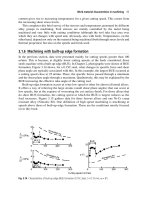
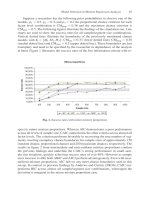
to be the first order CRF with a shift of 2. For this setting, Figure 1 presents the
results in terms of precision, recall and F1.
What can be observed not only from Figure 1 but also for all parameter settings
is the following: Using unsupervised tags as features as compared to no tagging
leads to a slightly decreased precision but a substantial increase in recall, and always
affects the F1 measure positively. The reason can be sought in the generalization
power of the tagger: having at hand syntactic-semantic tags instead of merely plain
words, the system is able to classify more instances correctly, as the tag (but not the
word) has occurred with the correct classification in the training set before. Due to
overgeneralization or tagging errors, however, precision is decreased. The effect is
Supporting Web-based Address Extraction with Unsupervised Tagging 583
Fig. 1. Results in precision, recall and F1 for all classes, obtained with first order CRF and a

shift of 2.
strongest for
street
with a loss of 7% in precision with a recall boost of 14%.
In general, unsupervised tagging clearly helps at this task, as a little loss in precision
is more than compensated with a boost in recall.
5 Conclusion and further work
In this research we have shown that the use of large, unannotated text can improve
classification results on small, manually annotated training sets via building a tag-
ger model with unsupervised tagging and using the unsupervised tags as features in
the learning algorithm. The benefit of unsupervised tagging is especially significant
in domain-specific settings, where standard pre-processing steps such as supervised
tagging do not capture the abstraction granularity necessary for the task, or simply no
tagger for the target language is available. For further work, we aim at combining the
possibly several addresses per target location. Given the evaluation values obtained
with our method, the task of dynamically extracting addresses from web-pages to
support address search for the tourist domain is feasible and a valuable, dynamic
add-on to directory-based address search.
References
BIEMANN, C. (2006a): Unsupervised Part-of-Speech Tagging Employing Efficient Graph
Clustering. Proc. COLING/ACL-06 SRW, Sydney, Australia.
BIEMANN, C. (2006b): Chinese Whispers - an Efficient Graph Clustering Algorithm and its
Application to Natural Language Processing Problems. Proceedings of the HLT-NAACL-
06 Workshop on Textgraphs, New York, USA.
584 Berenike Loos and Chris Biemann
DUNNING, T. (1993): Accurate Methods for the Statistics of Surprise and Coincidence. Com-
putational Linguistics 19(1), pp. 61–74.
FAULHABER A., LOOS B., PORZEL R., MALAKA, R. (2006): Towards Understanding the
Unknown: Open-class Named Entity Classification in Multiple Domains. Proceedings of
the Ontolex Workshop at LREC, Genova, Italy

FREITAG, D. (2004): Toward unsupervised whole-corpus tagging. Proceedings of the 20th
International Conference on Computational Linguistics, Geneva, Switzerland
GRISHMAN, R. (1997): Information Extraction: Techniques and Challenges. In Maria Teresa
Pazienza (ed.) Information Extraction. Springer-Verlag, Lecture Notes in Artificial Intel-
ligence, Rome
LAFFERTY, J. and McCALLUM, A. K. and PEREIRA, F. (2001): Conditional random fields:
Probabilistic models for segmenting and labeling sequence data. Proceedings of ICML-
01, pp. 282–289.
LOOS, B. (2006): On2L – A Framework for Incremental Ontology Learning in Spoken Dialog
Systems. Proc. COLING/ACL-06 SRW, Sydney, Australia
MCCALLUM, A. K. (2002): MALLET: A Machine Learning for Language Toolkit.
.
QUASTHOFF, U., RICHTER, M. and BIEMANN, C. (2006): Corpus Portal for Search in
Monolingual Corpora. Proceedings of LREC-06, Genoa, Italy
ROTH, D. and VAN DEN BOSCH, A. (Eds.) (2002): Proceedings of the Sixth Workshop on
Computational Language Learning (CoNNL-02), Taipei, Taiwan.
SARKAR, A. and HAFFARI, G. (2006): Inductive Semi-supervised Learning Methods for
Natural Language Processing. Tutorial at HLT-NAACL-06, NYC, USA.
SCHÜTZE, H. (1995): Distributional part-of-speech tagging. Proceedings of the 7th Con-
ference on European chapter of the Association for Computational Linguistics, Dublin,
Ireland
VAN RIJSBERGEN, C. J. (1979): Information Retrieval, 2nd edition. Dept. of Computer
Science, University of Glasgow.
Text Mining of
Supreme Administrative Court Jurisdictions
Ingo Feinerer and Kurt Hornik
Department of Statistics and Mathematics,
Wirtschaftsuniversität Wien, A-1090 Wien, Austria
{h0125130, Kurt.Hornik}@wu-wien.ac.at
Abstract. Within the last decade text mining, i.e., extracting sensitive information from text

corpora, has become a major factor in business intelligence. The automated textual analysis of
law corpora is highly valuable because of its impact on a company’s legal options and the raw
amount of available jurisdiction. The study of supreme court jurisdiction and international law
corpora is equally important due to its effects on business sectors.
In this paper we use text mining methods to investigate Austrian supreme administra-
tive court jurisdictions concerning dues and taxes. We analyze the law corpora using
R with
the new text mining package tm. Applications include clustering the jurisdiction documents
into groups modeling tax classes (like income or value-added tax) and identifying jurisdiction
properties. The findings are compared to results obtained by law experts.
1 Introduction
A thorough discussion and investigation of existing jurisdictions is a fundamental ac-
tivity of law experts since convictions provide insight into the interpretation of legal
statutes by supreme courts. On the other hand, text mining has become an effective
tool for analyzing text documents in automated ways. Conceptually, clustering and
classification of jurisdictions as well as identifying patterns in law corpora are of key
interest since they aid law experts in their analyses. E.g., clustering of primary and
secondary law documents as well as actual law firm data has been investigated by
Conrad et al. (2005). Schweighofer (1999) has conducted research on automatic text
analysis of international law.
In this paper we use text mining methods to investigate Austrian supreme ad-
ministrative court jurisdictions concerning dues and taxes. The data is described in
Section 2 and analyzed in Section 3. Results of applying clustering and classifica-
tion techniques are compared to those found by tax law experts. We also propose
a method for automatic feature extraction (e.g., of the senate size) from Austrian
supreme court jurisdictions. Section 4 concludes.
570 Ingo Feinerer and Kurt Hornik
2 Administrative Supreme Court jurisdictions
2.1 Data
The data set for our text mining investigations consists of 994 text documents. Each

document contains a jurisdiction of the Austrian supreme administrative court (Ver-
waltungsgerichtshof, VwGH) in German language. Documents were obtained
through the legal information system (Rechtsinformationssystem, RIS;
http://ris.
bka.gv.at/
) coordinated by the Austrian Federal Chancellery. Unfortunately, docu-
ments delivered through the RIS interface are HTML documents oriented for browser
viewing and possess no explicit metadata describing additional jurisdiction details
(e.g., the senate with its judges or the date of decision). The data set corresponds to
a subset of about 1000 documents of material used for the research project “Analyse
der abgabenrechtlichen Rechtsprechung des Verwaltungsgerichtshofes” supported
by a grant from the Jubiläumsfonds of the Austrian National Bank (Oesterreichische
Nationalbank, OeNB), see Nagel and Mamut (2006). Based on the work of Achatz
et al. (1987) who analyzed tax law jurisdictions in the 1980s this project investigates
whether and how results and trends found by Achatz et al. compare to jurisdictions
between 2000 and 2004, giving insight into legal norm changes and their effects
and unveiling information on the quality of executive and juristic authorities. In the
course of the project, jurisdictions especially related to dues (e.g., on a federal or
communal level) and taxes (e.g., income, value-added or corporate taxes) were clas-
sified by human tax law experts. These classifications will be employed for validating
the results of our text mining analyses.
2.2 Data preparation
We use the open source software environment
R for statistical computing and graph-
ics, in combination with the
R text mining package tm to conduct our text mining ex-
periments.
R provides premier methods for clustering and classification whereas tm
provides a sophisticated framework for text mining applications, offering functional-
ity for managing text documents, abstracting the process of document manipulation

and easing the usage of heterogeneous text formats.
Technically, the jurisdiction documents in HTML format were downloaded
through the RIS interface. To work with this inhomogeneous set of malformed HTML
documents, HTML tags and unnecessary white space were removed resulting in
plain text documents. We wrote a custom parsing function to handle the automatic
import into tm’s infrastructure and extract basic document metadata (like the file
number).
3 Investigations
3.1 Grouping the jurisdiction documents into tax classes
When working with larger collections of documents it is useful to group these into
clusters in order to provide homogeneous document sets for further investigation by
Text Mining of Supreme Administrative Court Jurisdictions 571
experts specialized on relevant topics. Thus, we investigate different methods known
in the text mining literature and compare their results with the results found by law
experts.
k-means Clustering
We start with the well known k-means clustering method on term-document ma-
trices. Let tf
t,d
be the frequency of term t in document d, m the number of docu-
ments, and df
t
is the number of documents containing the term t. Term-document
matrices M with respective entries Z
t,d
are obtained by suitably weighting the term-
document frequencies. The most popular weighting schemes are Term Frequency
(tf ), where Z
t,d
= tf

t,d
,andTerm Frequency Inverse Document Frequency (tf-idf ),
with Z
t,d
= tf
t,d
log
2
(m/df
t
), which reduces the impact of irrelevant terms and high-
lights discriminative ones by normalizing each matrix element under consideration
of the number of all documents. We use both weightings in our tests. In addition,
text corpora were stemmed before computing term-document matrices via the Rstem
(Temple Lang, 2006) and Snowball (Hornik, 2007)
R packages which provide the
Snowball stemming (Porter, 1980) algorithm.
Domain experts typically suggest a basic partition of the documents into three
classes (income tax, value-added tax, and other dues). Thus, we investigated the ex-
tent to which this partition is obtained by automatic classification. We used our data
set of about 1000 documents and performed k-means clustering, for k ∈{2, ,10}.
The best results were in the range between k = 3andk = 6 when considering the im-
provement of the within-cluster sum of squares. These results are shown in Table 1.
For each k, we compute the agreement between the k-means results based on the
term-document matrices with either tf or tf-idf weighting and the expert rating into
the basic classes, using both the Rand index (Rand) and the Rand index corrected for
agreement by chance (cRand). Row “Average” shows the average agreement over
the four ks. Results are almost identical for the two weightings employed. Agree-
Table 1. Rand index and Rand index corrected for agreement by chance of the contingency
tables between k-means results, for k ∈{3, 4,5,6}, and expert ratings for tf and tf-idf weight-

ings.
Rand cRand
k
tf tf-idf tf tf-idf
3 0.48 0.49 0.03 0.03
4
0.51 0.52 0.03 0.03
5
0.54 0.53 0.02 0.02
6
0.55 0.56 0.02 0.03
Average 0.52 0.52 0.02 0.03
ments are rather low, indicating that the “basic structure” can not easily be captured
by straightforward term-document frequency classification.
We note that clustering of collections of large documents like law corpora presents
formidable computational challenges due to the dimensionality of the term-document
572 Ingo Feinerer and Kurt Hornik
matrices involved: even after stopword removal and stemming, our about 1000 docu-
ments contained about 36000 different terms, resulting in (very sparse) matrices with
about 36 million entries. Computations took only a few minutes in our cases. Larger
datasets as found in law firms will require specialised procedures for clustering high-
dimensional data.
Keyword based Clustering
Based on the special content of our jurisdiction dataset and the results from k-means
clustering we developed a clustering method which we call keyword based cluster-
ing. It is inspired by simulating the behaviour of tax law students preprocessing the
documents for law experts. Typically the preprocessors skim over the text looking for
discriminative terms (i.e., keywords). Basically, our method works in the same way:
we have set up specific keywords describing each cluster (e.g., “income” or “income
tax” for the income tax cluster) and analyse each document on the similarity with the

set of keywords.
Experts
Keyword
ŦBased
N
one
I
ncome
t
ax
VA

t
ax
N
one
I
ncome tax
VA
tax
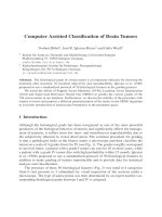
Fig. 1. Plot of the contingency table between the keyword based clustering results and the
expert rating.
Figure 1 shows a mosaic plot for the contingency table of cross-classifications of
keyword based clustering and expert ratings. The size of the diagonal cells (visual-
izing the proportion of concordant classifications) indicates that the keyword based
clustering methods works considerably better than the k-means approaches, with a
Text Mining of Supreme Administrative Court Jurisdictions 573
Rand index of 0.66 and a corrected Rand index of 0.32. In particular, the expert
“income tax” class is recovered perfectly.
3.2 Classification of jurisdictions according to federal fiscal code regulations

A further rewarding task for automated processing is the classification of jurisdic-
tions into documents dealing and into documents not dealing with Austrian federal
fiscal code regulations (Bundesabgabenordnung, BAO).
Due to the promising results obtained with string kernels in text classification and
text clustering (Lodhi et al., 2002; Karatzoglou and Feinerer, 2007) we performed a
“C-svc” classification with support vector machines using a full string kernel, i.e.,
using
k(x, y)=

s∈6
∗
O
s
·Q
s
(x) ·Q
s
(y)
as the kernel function k(x,y) for two character sequences x and y. We set the decay
factor O
s
= 0 for all strings |s|> n, where n denotes the document lengths, to instan-
tiate a so-called full string kernel (full string kernels are computationally much better
natured). The symbol 6
∗
is the set of all strings (under the Kleene closure), and Q
s
(x)
denotes the number of occurrences of s in x.
For this task we used the kernlab (Karatzoglou et al., 2006; Karatzoglou et

al., 2004)
R package which supports string kernels and SVM enabled classification
methods. We used the first 200 documents of our data set as training set and the next
50 documents as test set. We compared the 50 received classifications with the ex-
pert ratings which indicate whether a document deals with the BAO by constructing
a contingency table (confusion matrix). We received a Rand index of 0.49. After cor-
recting for agreement by chance the Rand index floats around at 0. We measured a
very long running time (almost one day for the training of the SVM, and about 15
minutes prediction time per document on a 2.6 GHz machine with 2 GByte RAM).
Therefore we decided to use the classical term-document matrix approach in ad-
dition to string kernels. We performed the same set of tests with tf and tf-idf weight-
ing, where we used the first 200 rows (i.e, entries in the matrix representing docu-
ments) as training set, the next 50 rows as test set.
Table 2. Rand index and Rand index corrected for agreement by chance of the contingency
tables between SVM classification results and expert ratings for documents under federal fiscal
code regulations.
tf tf-idf
Rand 0.59 0.61
cRand
0.18 0.21
Table 2 presents the results for classifications obtained with both tf and tf-idf
weightings. We see that the results are far better than the results obtained by employ-
ing string kernels.
574 Ingo Feinerer and Kurt Hornik
These results are very promising, and indicate the great potential of employing
support vector machines for the classification of text documents obtained from ju-
risdictions in case term-document matrices are employed for representing the text
documents.
3.3 Deriving the senate size
Table 3. Number of jurisdictions ordered by senate size obtained by fully automated text

mining heuristics. The percentage is compared to the percentage identified by humans.
Senate size
03 59
Documents 0 255 739 0
Percentage
0.000 25.654 74.346 0.000
Human Percentage
2.116 27.306 70.551 0.027
Jurisdictions of the Austrian supreme administrative court are obtained in so-
called senates which can have 3, 5, or 9 members, with size indicative of the “diffi-
culty” of the legal case to be decided. (It is also possible that no senate is formed.) An
automated derivation of the senate size from jurisdiction documents would be highly
useful, as it would allow to identify structural patterns both over time and across
areas. Although the formulations describing the senate members are quite standard-
ized it is rather hard and time-consuming for a human to extract the senate size from
hundreds of documents because a human must read the text thoroughly to differ be-
tween senate members and auxiliary personnel (e.g., a recording clerk). Thus, a fully
automated extraction would be very useful.
Since most documents contain standardized phrases regarding senate members
(e.g., “The administrative court represented by president Dr. X and the judges Dr.
YandDr.Z decided ”)wedeveloped an extractionheuristicbasedonwidely
used phrases in the documents to extract the senate members. In detail, we investigate
punctuation marks and copula phrases to derive the senate size. Table 3 summarizes
the results for our data set by giving the total number of documents for senate sizes
of zero (i.e., documents where no senate was formed, e.g., due to dismissal for want
of form), three, five, or nine members. The table also shows the percentages and
compares these to the aggregated percentages of the full data set, i.e., n > 1000,
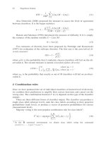
found by humans. Figure 2 visualizes the results from the contingency table between
machine and human results in form of an agreement plot, where the observed and ex-
pected diagonal elements are represented by superposed black and white rectangles,

respectively. The plot indicates that the extraction heuristic works very well. This is
supported by the very high Rand index of 0.94 and by the corrected Rand index of
0.86.
Further improvements could be achieved by saving identified names of judges in
order to identify them again in other documents. Of course, ideally information such
as senate size would be provided as metadata by the legal information system, per-
Text Mining of Supreme Administrative Court Jurisdictions 575
haps even determined automatically by text mining methods for “most” documents
(with a per-document measure of the need for verification by humans).
Human
Machine
0
0
3
3
5
5
Fig. 2. Agreement plot of the contingency table between the senate size reported by text min-
ing heuristics and the senate size reported by humans.
4 Conclusion
In this paper we have presented approaches to use text mining methods on (supreme
administrative) court jurisdictions. We performed k-means clustering and introduced
keyword based clustering which works well for text corpora with well defined formu-
lations as found in tax law related jurisdictions. We saw that the clustering works well
enough to be used as a reasonable grouping for further investigation by law experts.
Second, we investigated the classification of documents according to their relation to
federal fiscal code regulations. We used both string kernels and term-document ma-
trices with tf and tf-idf weighting as input for support vector machine based classifi-
cation techniques. The experiments unveiled that employing term-document matrices
yields both superior performance as well as fast running time. Finally, we considered

a situation typical in working with specialized text corpora, i.e., we were looking for
a specific property in each text corpus. In detail we derived the senate size of each ju-
risdiction by analyzing relevant text phrases considering punctuation marks, copulas
and regular expressions. Our results show that text mining methods can clearly aid
legal experts to process and analyze their law document corpora, offering both con-
siderable savings in time and cost as well as the possibility to conduct investigations
barely possible without the availability of these methods.
576 Ingo Feinerer and Kurt Hornik
Acknowledgments
We would like to thank Herbert Nagel for providing us with information and giving
us feedback.
References
ACHATZ, M., KAMPER, K., and RUPPE H. (1987): Die Rechtssprechung des VwGH in
Abgabensachen. Orac Verlag, Wien.
CONRAD, J., AL-KOFAHI, K., ZHAO, Y. and KARYPIS, G. (2005): Effective Document
Clustering for Large Heterogeneous Law Firm Collections. In: 10th International Con-
ference on Artificial Intelligence and Law (ICAIL). 177–187.
FEINERER, I. (2007): tm: Text Mining Package,
R package version 0.1-2.
HORNIK, K. (2007): Snowball: Snowball Stemmers,
R package version 0.0-1.
KARATZOGLOU, A. and FEINERER, I. (2007): Text Clustering with String Kernels in
R.
In: Advances in Data Analysis (Proceedings of the 30th Annual Conference of the GfKl).
91–98. Springer-Verlag.
KARATZOGLOU, A., SMOLA, A. and HORNIK, K. (2006): kernlab: Kernel-based machine
learning methods including support vector machines,
R package version 0.9-1.
KARATZOGLOU, A., SMOLA, A., HORNIK, K. and ZEILEIS, A. (2004): kernlab —An
S4 Package for Kernel Methods in

R. Journal of Statistical Software, 11(9), 1–20.
LODHI, H., SAUNDERS, C., SHAWE-TAYLOR, J., WATKINS, C., and CRISTIANINI, N.
(2002): Text classification using string kernels. Journal of Machine Learning Research,
2, 419–444.
NAGEL, H. and MAMUT, M. (2006): Rechtsprechung des VwGH in Abgabensachen 2000–
2004.
PORTER, M. (1980): An algorithm for suffix stripping. Program, 14(3), 130–137.
R DEVELOPMENT CORE TEAM (2006): R: A Language and Environment for Statistical
Computing.
R Foundation for Statistical Computing, Vienna, Austria. ISBN 3-900051-
07-0, URL
/>.
SCHWEIGHOFER, E. (1999): Legal Knowledge Representation, Automatic Text Analysis in
Public International and European Law. Kluwer Law International, Law and Electronic
Commerce, Volume 7, The Hague. ISBN 9041111484.
TEMPLE LANG, D. (2006): Rstem: Interface to Snowball implementation of Porter’s word
stemming algorithm,
R package version 0.3-1.
Projecting Dialect Distances to Geography: Bootstrap
Clustering vs. Noisy Clustering
John Nerbonne
1
, Peter Kleiweg
1
, Wilbert Heeringa
1
and Franz Manni
2
1
Alfa-informatica, University of Groningen, Netherlands

{j.nerbonne, p.c.j.kleiweg, w.j.heeringa}@rug.nl
2
Musée de l’Homme, Paris, France

Abstract. Dialectometry produces aggregate DISTANCE MATRICES in which a distance is
specified for each pair of sites. By projecting groups obtained by clustering onto geography
one compares results with traditional dialectology, which produced maps partitioned into im-
plicitly non-overlapping
DIALECT AREAS. The importance of dialect areas has been chal-
lenged by proponents of
CONTINUA, but they too need to compare their findings to older
literature, expressed in terms of areas.
Simple clustering is unstable, meaning that small differences in the input matrix can lead
to large differences in results (Jain et al. 1999). This is illustrated with a 500-site data set from
Bulgaria, where input matrices which correlate very highly (r = 0.97) still yield very different
clusterings. Kleiweg et al. (2004) introduce
COMPOSITE CLUSTERING, in which random noise
is added to matrices during repeated clustering. The resulting borders are then projected onto
the map.
The present contribution compares Kleiweg et al.’s procedure to resampled bootstrapping,
and also shows how the same procedure used to project borders from composite clustering
may be used to project borders from bootstrapping.
1 Introduction
We focus on dialectal data, examined at a high level of aggregation, i.e. the average
linguistic distance between all pairs of sites in large dialect surveys. It is important
to seek groups in this data, both to examine the importance of groups as organizing
elements in the dialect landscape, but also in order to compare current, computa-
tional work to traditional accounts. Clustering is thus important as a means of seek-
ing groups in data, but it suffers from instability: small input differences can lead to
large differences in results, i.e., in the groups identified.

We investigate two techniques for overcoming the instability in clustering tech-
niques, bootstrapping, well known from the biological literature, and “noisy” clus-
tering, which we introduce here. In addition we examine a novel means of projecting
the results of (either technique involving) such repeated clusterings to the geographic
648 John Nerbonne, Peter Kleiweg, Wilbert Heeringa and Franz Manni
map, arguing that it is better suited to revealing the detailed structure in dialectolog-
ical distance matrices.
2 Background and motivation
We assume the view of dialectometry (Goebl, 1984 inter alia) that we characterize
dialects in a given area in terms of an aggregate distance matrix, i.e. an assignment
of a linguistic distance d to each pair of sites s
1
,s
2
in the area D
l
(s
1
,s
2
)=d.Lin-
guistic distances may be derived from vocabulary differences, differences in struc-
tural properties such as syntax (Spruit, 2006), differences in pronunciation, or oth-
erwise. We ignore the derivation of the distances here, except to note two aspects.
First, we derive distances via individual linguistic items (in fact, words), so that we
are able to examine the effect of sampling on these items. Second, we focus on
true distances, satisfying the usual distance axioms, i.e. having a minimum at zero:
∀s
1
D(s

1
,s
1
)=0; symmetry: ∀s
1
,s
2
D(s
1
,s
2
)=D(s
2
,s
1
); and the triangle inequal-
ity: ∀s
1
s
2
s
3
D(s
1
,s
2
) ≤D(s
1
,s
3

)+D(s
3
,s
2
) (see (Kruskal 1999:22). We return to the
issue of whether the distances are
ULTRAMETRIC in the sense of the phylogenetic
literature below.
We focus here on how to analyze such distance matrices, and in particular how
to detect areas of relative similarity. While multi-dimensional scaling has undoubt-
edly proven its value in dialectometric studies (Embleton (1987), Nerbonne et al.
(1999)), we still wish to detect
DIALECT AREAS, both in order to examine how well
areas function as organizing entities in dialectology, and also in order to compare
dialectometric work to traditional dialectology in which dialect areas were seen as
the dominant organizing principle.
C
LUSTERING is a standard way in which to seek groups in such data, and it
is applied frequently and intelligently to the results of dialectometric analyses. The
research community is convinced that the linguistic varieties are hierarchically or-
ganized; thus, e.g., the urban dialect of Freiburg is a sort of Low Alemannic, which
is in turn Alemannic, which is in turn Southern German, etc. This means that the
techniques of choice have been different varieties of hierarchical clustering (Schiltz
(1996), Mucha and Haimerl (2005)).
Hierarchical clustering is most easily understood procedurally: given a square
distance matrix of size n ×n, we seek the smallest distance in it. Assume that this
is the distance between i and j. We then fuse the two elements i and j, obtaining an
n−1 square matrix. One needs to determine the distance from the newly added i+ j
element to all remaining k, and there are several alternatives for doing this, including
nearest neighbor, average distance, weighted average distance, and minimal variance

(Ward’s method). See Jain et al. (1999) for discussion. We return in the discussion
section to the differences between the clustering algorithms, but in order to focus on
the effects of bootstrapping and “noisy” clustering, we use only weighted average
(WPGMA) in the experiments below.
The result of clustering is a
DENDROGRAM, a tree in which the history of the
clustering may be seen. For any two leaf nodes in the dendrogram we may determine
Projecting Dialect Distances to Geography 649
Bockelwitz
Schmannewitz
Borstendorf
Gornsdorf
Wehrsdorf
Cursdorf
0.03 0.04 0.05
Fig. 1. An Example Dendrogram. Note the cophenetic distance is reflected in the horizontal
distance from the leaves to the encompassing node. Thus the cophenetic distance between
Borstendorf and Gornsdorf is a bit more than 0.04.
the point at which they fuse, i.e. the smallest internal node which contains them
both. In addition, we record the
COPHENETIC DISTANCE: this is the distance from
one subnode to another at the point in the algorithm at which the subnodes fused.
Note that the algorithms depend on identifying minimal elements, which leads to
instability: small changes in the input data can lead to very different groups’ being
identified (Jain et al., 1999). Nor is this problem merely “theoretical”. Figure 2 shows
two very different cluster results which from genuine, extremely similar data (the
distance matrices correlated at r = 0.97).
Fig. 2. Two Bulgarian Datasets from Osenova et al. (to appear). Although the distance matrices
correlated nearly perfectly (r = 0.97), the results of WPGMA clustering differ substantially.
Bootstrapping and noisy clustering resolve this instability.

Finally, we note that the distances we shall cluster do not satisfy the ultrametric
axiom: ∀s
1
s
2
s
3
D(s
1
,s
2
) ≤ max{D(s
2
,s
3
),D(s
1
,s
3
)} (Page and Holmes (2006:26)).
Phylogeneticists interpret data satisfying this axiom temporally, i.e., they interpret
data points clustered together as later branches in an evolutionary tree. The dialec-
tal data undoubtedly reflects historical developments to some extent, but we proceed
from the premise that the social function of dialect variation is to signal geographic
provenance, and that similar linguistic variants signal similar provenance. If the sig-
nal is subject to change due to contact or migration, as it undoubtedly is, then sim-
ilarity could also result from recent events. This muddies the history, but does not
change the socio-geographic interpretation.
650 John Nerbonne, Peter Kleiweg, Wilbert Heeringa and Franz Manni
2.1 Data

In the remainder of the paper we use the data analyzed by Nerbonne and Siedle
(2005) consisting of 201 word pronunciations recorded and transcribed at 186 sites
throughout all of contemporary Germany. The data was collected and transcribed
by researchers at Marburg between 1976 and 1991. It was digitized and analyzed
in 2003–2004. The distance between word pronunciations was measured using a
modified version of edit distance, and full details (including the data) are available.
See Nerbonne and Siedle (2005).
3 Bootstrapping clustering
The biological literature recommends the use of bootstrapping in order to obtain
stable clustering results (Felsenstein, 2004: Chap. 20). Mucha and Haimerl (2005)
and Manni et al. (2006) likewise recommend bootstrapping for the interpretation of
clustering applied to dialectometric data.
In bootstrapped clustering we resample the data, using replacement. In our case
we resample the set of word-pronunciation distances. As noted above, each linguis-
tic observation o is associated with a site×site matrix M
o
. In the observation matrix,
each cell represents the linguistic distance between two sites with respect to the ob-
servation: M
o
(s,s

)=D(o
s
,o
s

). In bootstrapping, we assign a weight to each matrix
(observation) identical to the number of times it is chosen in resampling:
w

o
=

n if observation o is drawn n times
0otherwise
If we resample I times, then I =

o
w
o
. The result is a subset of the original set of
observations (words), where some of the observations may be weighted as a resulted
of the resampling. Each resampled set of words yields a new distance matrix M
i∈I
,
namely the average distances of the sites using the weighted set of words obtained
via bootstrapping.
We apply clustering to each M
i
obtained via bootstrapping, recording for each
group of sites encountered in the dendrogram (each set of leaves below some node)
both that the group was encountered, and the cophenetic distance of the group (at
the point of fusion). This sounds as if it could lead to a combinatorial problem, but
fortunately most of the 2
180
possible groups are never encountered.
In a final step we extract a
COMPOSITE DENDROGRAM from this collection,
consisting of all of the groups that appear in a majority of the clustering iterations,
together with their cophenetic distance. See Fig. 3 for an example.

4 Clustering with noise
Clustering with noise is also motivated by the wish to prevent the sort of instability
illustrated in Fig. 2. To cluster with noise we assume a single distance matrix, from
Projecting Dialect Distances to Geography 651
which it turns out to be convenient to calculate variance (among all the distances).
We then specify a small noise ceiling c, e.g. c = V/2, i.e. one-half standard deviation
of distances in the matrix. We then repeat 100 times or more: add random amounts
of noise r to the matrix (i.e., different amounts to each cell), allowing r to vary
uniformly, 0 ≤r ≤ c.
Altenberg
Schraden
54
Bockelwitz
Schmannewitz
97
Linz
60
Grünlichtenberg
Roßwein
100
69
Lampertswalde
72
Jonsdorf
Rammenau
88
Gersdorf
72
65
Altlandsberg

Lippen
100
Groß Jamno
100
Pretzsch
100
Neu Schadow
93
Gerbstedt
Landgrafroda
100
53
Borstendorf
Gornsdorf
100
Theuma
96
Mockern
55
Cursdorf
Osterfeld
Wehrsdorf
56
Fig. 3. A Composite Dendrogram where labels indicate how often a groups of sites was clus-
tered and the (horizontal) length of the brackets reflects mean cophenetic distance.
If we let M
i
stand in this case for the matrix obtained by adding noise (in the i-th
iteration), then the rest of the procedure is identical to bootstrapping. We apply clus-
tering to M

i
and record the groups clustered together with their cophenetic distances,
just as in Fig. 3.
5 Projecting to geography
Since dialectology studies the geographic variation of language, it is particularly
important to be able to examine the results of analyses as these correspond to geog-
raphy.
In order to project the results of either bootstrapping or noisy clustering to the
geographic map, we use the customary Voronoi tessellation (Goebl (1984)), in which
each site is embedded in a polygon which separates it from other sites optimally. In
this sort of tiling there is exactly one border running between each pair of adjacent
sites, and bisecting the imaginary line linking the two. To project mean cophenetic
distance matrices onto the map we simply draw the Voronoi tessellation in such a
way that the darkness of each line corresponds to the distance between the two sites
it separates. See Fig. 4 for examples of maps obtained by bootstrapping two different
clustering algorithms. These largely corroborate scholarship on German dialectology
(König 1991:230–231).
Unlike dialect area maps these
COMPOSITE CLUSTER MAPS reflect the variable
strength of borders, represented by the border’s darkness, reflecting the consensus
cophenetic distance between the adjacent sites.
Haag (1898) (discussed by Schiltz (1996)) proposed a quantitative technique in
which the darkness of a border was reflected by the number of differences counted in
652 John Nerbonne, Peter Kleiweg, Wilbert Heeringa and Franz Manni
a given sample, and similar maps have been in use since. Such maps look similar to
the maps we present here, but note that the borders we sketch need not be reflected in
local differences between the two sites. The clustering can detect borders even where
differences are gradual, when borders emerge only when many sites are compared.
1
6 Results

Bootstrapping clustering and “noisy” clustering identify the same groups in the 186-
site German sample examined here. This is shown by the nearly perfect correlation
between the mean cophenetic distances assigned by the two techniques (r = 0.997).
Given the general acceptance of bootstrapping as a means of examining the stability
of clusters, this result shows that “noisy” clustering is as effective.
The usefulness of the composite cluster map may best be appreciated by inspect-
ing the maps in Fig. 4. While maps projected from simple clustering (see Fig. 2)
merely partition an area into non-overlapping subareas, these composite maps re-
flect a great deal more of the detailed structure in the data. The map on the left was
obtained by bootstrapping using WPGMA.
Although both bootstrapping and adding noise identifies stable groups, neither
removes the bias of the particular clustering algorithm. Fig. 4 compares the boot-
strapped results of WPGMA clustering with unweighted clustering (UPGMA, see
Jain (1999)). In both cases bootstrapping and noisy clustering correlate nearly per-
fectly, but it is clear that the WPGMA is sensitive to more structure in the data.
For example, it distinguishes Bavaria (in southeastern Germany) from the Southwest
(Swabia and Alemania). So the question of the optimal clustering method for dialec-
tal data remains. For further discussion see
/>kaarten/MDS-clusters.html
.
7 Discussion
The “noisy”clustering examined here requires that one specify a parameter, the noise
ceiling, and, naturally, one prefers to avoid techniques involving extra parameters.
On the other hand it is applicable to single matrices, unlike bootstrapping, which
requires that one be able to identify components to be selected in resampling. Both
techniques require that one specify a number of iterations, but this is a parameter of
convenience. Small numbers of iterations are convenient, and large values result in
very stable groupings.
1
Fischer (1980) discusses adding a contiguity constraint to clustering, which structures the

hypothesis space in a way that favors clusterings of contiguous regions. Since we use the
projection to geography to spot linguistic anomalies—dialect islands, but also field worker
and transcriber errors—we do not wish to push the clustering in a direction that would hide
these anomalies.
Projecting Dialect Distances to Geography 653
Fig. 4. Two Composite Cluster Maps, on the left one obtained by bootstrapping using weighted
group average clustering, and on the right one obtained by unweighted group average. We do
not show the maps obtained using “noisy” clustering, as these are indistinguishable from the
maps obtained via bootstrapping. The composite distance matrices correlate nearly perfectly
(r = 0.997) when comparing bootstrapping and “noisy” clustering.
Acknowledgments
We are grateful to Rolf Backofen, Hans Holm and Wilbert Heeringa for discussion,
to Hans-Joachim Mucha and Edgar Haimerl for making their 2007 paper available
before GfKl 2007, and to two anonymous GfKl referees.
References
EMBLETON, S. (1987): Multidimensional Scaling as a Dialectometrical Technique. In: R.
M. Babitch (Ed.) Papers from the Eleventh Annual Meeting of the Atlantic Provinces
Linguistic Association, Centre Universitaire de Shippagan, New Brunswick, 33-49.
FELSENSTEIN, J. (2004): Inferring Phylogenies. Sinauer, Sunderland, MA.
FISCHER, M. (1980): Regional Taxonomy: A Comparison of Some Hierarchic and Non-
Hierarchic Strategies. Regional Science and Urban Economics 10, 503–537.
GOEBL, H. (1984): Dialektometrische Studien: Anhand italoromanischer, rätoromanischer
und galloromanischer Sprachmaterialien aus AIS und ALF 3 Vol. Max Niemeyer, Tübin-
gen.
HAAG, K. (1898): Die Mundarten des oberen Neckar- und Donaulandes. Buchdruckerei Egon
Hutzler, Reutlingen.
654 John Nerbonne, Peter Kleiweg, Wilbert Heeringa and Franz Manni
JAIN, A. K., MURTY, M. N., and FLYNN, P. J. (1999): Data Clustering: A Review. ACM
Computing Surveys 31(3), 264–323.
KLEIWEG, P., NERBONNE, J. and BOSVELD, L. (2004): Geographic Projection of Cluster

Composites. In: A. Blackwell, K. Marriott and A. Shimojima (Eds.) Diagrammatic Rep-
resentation and Inference. 3rd Intn’l Conf, Diagrams 2004. Cambridge, UK, Mar. 2004.
(Lecture Notes in Artificial Intelligence 2980). Springer, Berlin, 392-394.
KÖNIG, W. (1991,
1
1978): DTV-Atlas zur detschen Sprache. DTV, München.
KRUKSAL, J. (1999): An Overview of Sequence Comparison. In: D. Sankoff and J. Kruskal
(Eds.) Time Warps, String Edits and Macromolecules: The Theory and Practice of Se-
quence Comparison, 2nd ed. CSLI, Stanford, 1–44.
MANNI, F. HEERINGA, W. and NERBONNE, J. (2006): To what Extent are Surnames
Words? Comparing Geographic Patterns of Surnames and Dialect Variation in the Nether-
lands. In Literary and Linguistic Computing 21(4), 507-528.
MUCHA, H.J. and HAIMERL, E. (2005): Automatic Validation of Hierarchical Cluster Anal-
ysis with Application in Dialectometry. In: C. Weihs and W. Gaul (Eds.) Classification—
the Ubiquitous Challenge. Proc. of 28th Mtg Gesellschaft für Klassifikation, Dortmund,
Mar. 9–11, 2004. Springer, Berlin, 513–520.
NERBONNE, J., HEERINGA, W. and KLEIWEG, P. (1999): Edit Distance and Dialect Prox-
imity. In: D. Sankoff and J. Kruskal (Eds.) Time Warps, String Edits and Macromolecules:
The Theory and Practice of Sequence Comparison, 2nd ed. CSLI, Stanford, v-xv.
NERBONNE, J. and SIEDLE, Ch. (2005): Dialektklassifikation auf der Grundlage ag-
gregierter Ausspracheunterschiede. Zeitschrift für Dialektologie und Linguistik 72(2),
129-147.
PAGE, R.D.M., and HOLMES, E.C. (2006): Molecular Evolution: A Phylogenetic Approach.
(
1
1998) Blackwell, Oxford.
SCHILTZ, G. (1996): German Dialectometry. In: H H. Bock and W. Polasek (Eds.) Data
Analysis and Information Systems: Statistical and Conceptual Approaches. Proc. of 19th
Mtg of Gesellschaft für Klassifikation, Basel, Mar. 8–10, 1995. Springer, Berlin, 526–
539.

SPRUIT, M. (2006): Measuring Syntactic Variation in Dutch Dialects. In J. Nerbonne and
W. Kretzschmar, Jr. (Eds.) Progress in Dialectometry: Toward Explanation. Special issue
of Literary and Linguistic Computing 21(4), 493–506.
Quantitative Text Analysis
Using L-, F- and T-Segments
Reinhard Köhler and Sven Naumann
Linguistische Datenverarbeitung, University of Trier, Germany
{koehler, naumsven}@uni-trier.de
Abstract. It is shown that word length and other properties of linguistic units display a lawful
behavior not only in form of distributions but also with respect to their syntagmatic arrange-
ment in a text. Based on L-segments (units of constant or increasing lengths), F-segments, and
T-segments (units of constant or increasing frequency or polytextuality respectively), the dy-
namic behavior of segment patterns is investigated. Theoretical models are derived on the basis
of plausible assumptions on influences of the properties of individual units on the properties
of their constituents in the text. The corresponding hypotheses are tested on data from 66 Ger-
man texts of four authors and two different genres. Experiments with various characteristics
show promising properties which could be useful for author and/or genre discrimination.
1 Introduction
Most quantitative studies in linguistics are almost exclusively based on a "bag of
words" model, i.e. they disregard the syntagmatic dimension, the arrangement of the
units in the course of the given text. Gustav Herdan underlined this fact as early as
1966; he called the two different types of study "language in the mass vs. language in
the line" (Herdan (1966), p. 423). Only very few investigations have been carried out
so far with respect to sequences of properties of linguistic units (cf. H
ˇ
rebí
ˇ
cek (2000),
Andersen (2005), Köhler (2006) and Uhlí
ˇ

rová (2007)). A special approach is time
series studies (cf. Pawlowski (2001)), but the application of such methods to studies
of natural language is not easy to justify and is connected with methodological prob-
lems of assigning numerical values to categorical observations. The present paper
approaches the problem of the dynamic behavior of sequences of properties without
limitation to a specific grouping such as word pairs or N-grams. It starts from the
general hypothesis that sequences in a text are organized in lawful patterns rather
than chaotically or according to a uniform distribution. There are several possibili-
ties to define units such as phrases or clauses which could be used to find patterns
or regularities. They suffer, however, from several disadvantages: (1) They do not
provide an appropriate granularity. While words are too small, sentences seem to be
too large units to unveil syntagmatic patterns with quantitative methods. (2) Linguis-
tic units are inherently connected to specific grammar models. (3) Their application
638 Reinhard Köhler and Sven Naumann
leads again to a "bag of units" model and thus to a loss of syntagmatic informa-
tion. Therefore, we establish a different unit for our present project: A unit based
on the rhythm of the property under study itself. We will demonstrate the approach
using word length as an illustrative example. We define an L-segment as a maxi-
mal sequence of monotonically increasing numbers, where these numbers represent
the lengths of adjacent words of the text. Using this definition, we segment a given
text in a left to right fashion starting with the first word. In this way, a text can be
represented as an uninterrupted sequence of L-segments. Thus, the text fragment (1)
is segmented as shown by the L-segment sequence (2)if word length is measured in
terms of syllable number:
(1) Word length studies are almost exclusively devoted to the
problem of distributions.
(2) (1-1-2) (1-2-4) (3) (1-1-2) (1-4)
This kind of segmentation is similar to Boroda’s F-motiv for musical "texts". Boroda
(1982) defined his F-motiv in an analogous way but with respect to the duration of
the notes of a musical piece. The advantage of such a definition is obvious: Any text

can be segmented in an objective, unambiguous, and exhaustive way, i.e. it guaranties
that each element will be assigned to exactly one unit. Furthermore, it provides units
of an appropriate granularity and it can be applied iteratively, i.e. sequences of L-
segments and their lengths can be studied etc., thus the unit can be scaled over a
principally unlimited range of sizes and granularities, limited only by text length.
Analogically, F- and T-segments are formed by monotonically increasing sequences
of frequency and polytextuality values. Other units than words can be used as basic
units, such as morphs, syllables, phrases, clauses, sentences, and other properties
such as polysemy, synonymy, age etc. can be used for analogous definitions. Our
study concentrated on L-, F-, and T-segments, and we will report here mainly on the
findings using L-segments. While the focus of our interest lies on basic scientific
questions such as "why do these units show their specific behavior?" we also had a
look at the possible use of our findings for purposes such as text genre classification
and authorship determination.
2 Data
For the present study we compiled a small corpus by selecting 66 documents from
the Projekt Gutenberg-DE ( The corpus consists of 30
poems and 36 short stories, written by 4 different German authors between the late
18th and the early 20th century:
Text length varies between 90 and 8500 running word forms (RWF). As to be
expected, the poems tend to be considerably shorter than the narrative texts: The
average length of the poems is 446 RWF and 3063 RWF of the short stories.