Conjoint Analysis for Complex Services Using Clusterwise HB Procedures 437
Table 3. Validity values for the total sample and for the clusters for HB estimation (“in to-
tal sample”: HB estimation at the individual total sample level; “in segment”: separate HB
estimation at the individual cluster 1 resp. 2 level)
Cluster 1 Cluster 2
Total sample (n=79)* (n=82)
(n=161)* In Total In In Total In
Sample Segment Sample Segment
First-choice-hit-rate
(using draws, n=10,000)
62.57 % 72.38 % 72.39 % 53.12 % 53.14 %
Mean Spearman
(using draws, n=10,000)
0.727 0.780 0.778 0.677 0.671
First-choice-hit-rate
(using mean draws)
65.22 % 75.95 % 74.68 % 54.88 % 57.32 %
Mean Spearman
(using mean draws)
0.748 0.802 0.797 0.696 0.700
* . . . one respondent had missing holdout data and could not be considered
considered. Furthermore we were interested whether clusterwise estimation can op-
timize the “results” of HB estimation. A clear answer is not possible up to now. In
our empirical investigation in some cases we had improvements with respect to the
validity values (cluster 2) and in some cases not (cluster 1).
This means that our proposition in the paper can help to reduce the problems that
occur when service preference measurement via conjoint analysis is the research
focus. HB estimation seems to improve validity even in case of complex services
with immaterial attributes and levels that cause perceptual uncertainty and preference
heterogeneity. However, going further with the more complicated way of performing
clusterwise HB estimation doesn’t provide automatically better results.

Nevertheless, further comparisons with larger sample sizes and other research ob-
jects are necessary. Furthermore, the possibilities of other validity criteria for clearer
statements could be used.
References
ALLENBY, G.M. and GINTER, J.L. (1995): Using Extremes to Design Products and Segment
Markets. Journal of Marketing Research, 32, November, 392–403.
ALLENBY, G.M., ARORA, N. and GINTER, J.L (1995): Incorporating Prior Knowledge into
the Analysis of Conjoint Studies. Journal of Marketing Research, 32, May, 152–162.
ANDREWS, R.L., ANSARI, A. and CURRIM, I.S. (2002): Hierarchical Bayes Versus Fi-
nite Mixture Conjoint Analysis Models: A Comparison of Fit, Prediction, and Partworth
Recovery. Journal of Marketing Research, 39, February, 87–98.
BAIER, D. and GAUL, W. (1999): Optimal Product Positioning Based on Paired Comparison
Data. Journal of Econometrics, 89, Nos. 1-2, 365–392.
438 Michael Brusch and Daniel Baier
BAIER, D. and GAUL, W. (2003): Market Simulation Using a Probabilistic Ideal Vector
Model for Conjoint Data. In: A. Gustafsson, A. Herrmann, and F. Huber (Eds.): Con-
joint Measurement - Methods and Applications. Springer, Berlin, 97–120.
BAIER, D. and POLASEK, W. (2003): Market Simulation Using Bayesian Procedures in
Conjoint Analysis. In: M. Schwaiger and O. Opitz (Eds.): Exploratory Data Analysis in
Empirical Research. Springer, Berlin, 413–421.
BRUSCH, M., BAIER, D. and TREPPA, A. (2002): Conjoint Analysis and Stimulus Presen-
tation - a Comparison of Alternative Methods. In: K. Jajuga, A. Sokođowski and H.H.
Bock (Eds.): Classification, Clustering, and Analysis. Springer, Berlin, 203–210.
ERNST, O. and SATTLER, H. (2000): Multimediale versus traditionelle Conjoint-Analysen.
Ein empirischer Vergleich alternativer Produktpräsentationsformen. Marketing ZFP, 2,
161–172.
GREEN, P.E. and SRINIVASAN, V. (1978): Conjoint Analysis in Consumer Research: Issues
and Outlook. Journal of Consumer Research, 5, September, 103–123.
GREEN, P.E., KRIEGER, A.M. and WIND, Y. (2001): Thirty Years of Conjoint Analysis:
Reflections and Prospects. Interfaces 31, 3, part 2, S56–S73.

LENK, P.J., DESARBO, W.S., GREEN, P.E. and YOUNG, M.R. (1996): Hierarchical Bayes
Conjoint Analysis: Recovery of Partworth Heterogeneity from Reduced Experimental
Designs. Marketing Science, 15, 2, 173–191.
LIECHTY, J.C., FONG, D.K.H. and DESARBO, W.S. (2005): Dynamic models incorporating
individual heterogeneity. Utility evolution in conjoint analysis. Marketing Science, 24,
285–293.
ORME, B. (2000): Hierarchical Bayes: Why All the Attention? Quirk’s Marketing Research
Review, March.
SAWTOOTH SOFTWARE (2002): ACA System. Adaptive Conjoint Analysis Version 5.0.
Technical Paper Series, Sawtooth Software.
SAWTOOTH SOFTWARE (2006): The ACA/Hierarchical Bayes v3.0 Technical Paper. Tech-
nical Paper Series, Sawtooth Software.
SENTIS, K. and LI, L. (2002): One Size Fits All or Custom Tailored: Which HB Fits Better?
Proceedings of the Sawtooth Software Conference September 2001, 167–175.
ZEITHAML, V.A., PARASURAMAN, A. and BERRY, L.L. (1985): Problems and Strategies
in Services Marketing. Journal of Marketing, 49, 33–46.
Heterogeneity in the Satisfaction-Retention
Relationship – A Finite-mixture Approach
Dorian Quint and Marcel Paulssen
Humboldt-Universität zu Berlin, Institut für Industrielles Marketing-Management,
Spandauer Str. 1, 10178 Berlin, Germany

,

Abstract. Despite the claim that satisfaction ratings are linked to actual repurchase behav-
ior, the number of studies that actually relate satisfaction ratings to actual repurchase behav-
ior is limited (Mittal and Kamakura 2001). Furthermore, in those studies that investigate the
satisfaction-retention link customers have repeatedly been shown to defect even though they
statetobehighlysatisfied. In a dramatic illustration of the problem Reichheld (1996) reports
that while around 90% of industry customers report to be satisfied or even very satisfied, only

between 30% to 40% actually repurchase. In this contribution, the relationship between satis-
faction and retention was examined using a sample of 1493 business clients in the market of
light transporters of a major European market. To examine heterogeneity in the satisfaction-
relationship, a finite-mixture approach was chosen to model a mixed logistic regression. The
subgroups found by the algorithm do differ with respect to the relationship between satisfac-
tion and loyalty, as well as with respect to the exogenous variables. The resulting model allows
us to shed more light on the role of the numerous moderating and interacting variables on the
satisfaction-loyalty link in a business-to-business context.
1 Introduction
It has been one of the fundamental assumptions of relationship marketing theory that
customer satisfaction has a positive impact on retention
1
. Satisfaction was supposed
to be the only necessary and sufficient condition for attitudinal loyalty (stated repur-
chase behavior) and the more manifest retention (actual repurchase behavior) and has
been used as an indicator for future profits (Reichheld 1996, Bolton 1998). However,
this seemingly undisputed relationship could not be fully confirmed by empirical
studies (Gremler and Brown 1996). Further research points out that there can be a
large gap between one-time satisfaction and repurchase behavior. Not always leads
an intention to repurchase (i.e. the statement in a questionnaire) to an actual repur-
chase and continuous repurchasing might exist without satisfaction because of mere
price settings (see Söderlund and Vilgon 1999, Morwitz 1997). What is more, only
1
I.e. Anderson et al. (2004), Bolton (1998), Söderlund and Vilgon (1999).
472 Dorian Quint and Marcel Paulssen
a small number of studies has actually examined repurchase behavior instead of the
easier to get repurchase intentions (Bolton 1998, Mittal and Kamakura 2001, Rust
and Zahorik 1993). The tenor of these studies is that the link between satisfaction
and retention is clearly weaker than the link between satisfaction and loyalty.
Many other factors were discovered to have an influence on retention. Also more

technical issues like common method variance, mere measurement effects or simply
unclear definitions added to raise doubt on the importance and the exact magnitude of
the contribution of satisfaction (Reichheld 1996, Söderlund/Vilgon 1999, Giese/Cote
2000). Another reason for the weak relationship between satisfaction and retention
is that it may not be a simple linear one, but one moderated by several different
variables. Several studies have already studied the effect of moderating variables on
the satisfaction-loyalty link (e.g. Homburg and Giering 2001). However, the great
majority of empirical studies in this field measured repurchase intentions instead
of objective repurchase behavior (Seiders et al. 2005). Thus, the conclusion from
prior work is that considerable heterogeneity is present that might explain the often
surprisingly weak overall relationship.
An important contribution has been put forth by Mittal and Kamakura (2001).
They combined the concepts of response biases and different thresholds
2
into their
model to capture individual differences between respondents. Based on their results
they created a customer group where repurchase behavior was completely unrelated
to levels of stated satisfaction. However, their approach fails to identify real existing
groups that have a distinctive relationship between satisfaction and retention. For ex-
ample, if model results show that older people have a lower threshold and thus repur-
chase with a higher probability given a certain level of satisfaction, this is not the full
story. Other factors, measured or unmeasured, might set off the age effect. In order
to find groups with distinctive relationships between satisfaction and retention, we
have explicitly chosen a finite-mixture
3
approach, which results in a mixed-logistic
regression setup. This model type basically consists of G logistic regressions – one
for each latent group. This way, each case i is assigned to a group with a unique
relation between the two constructs of interest. However, in a Bernoulli case like
this (see McLachlan and Peel 2000, p.163ff), identifiability is not given. The neces-

sary and sufficient condition for identifiability is G
max
≤
1
2
(m + 1), where m is the
number of Bernoulli trials. For m = 1 no ML-regression can be estimated. But Foll-
mann and Lambert (1991) prove theoretical identifiability of a special case of binary
ML-regressions. Only the thresholds O are allowed to vary over the groups, while
all remaining regression parameters are equal for all groups. According to Theorem
2 of Follmann and Lambert (1991) theoretical identifiability then depends only on
the maximal number of different values of one covariate N
max
given the values of all
other covariates are held constant. The maximal number of components is then given
by G
max
=
√
N
max
+ 2 −1. Thus, the theorem restricts the choice of the variables,
2
In our model thresholds are tolerance levels and can be conceived as the probability of
repurchase given all other covariates are zero.
3
For an overview on finite-mixture models, see McLachlan and Peel (2002) and the refer-
ences therein.
Heterogeneity in the Satisfaction-Retention Relationship 473
but ultimately helps building a suitable model for the relationship under investiga-

tion. In our final model we also included so-called concomitant covariate variables,
which help to understand latent class membership and enhance interpretability of
each group or class. This is achieved by using a multinomial regression of the latent
class variable c on these variables x:
P(c
gi
= 1|x
i
)=
e
D
g
+J

g
x
i

G
l=1
e
D
l
+J

l
x
i
=
e

D
g
+J

g
x
i
1+

G−1
l=1
e
D
l
+J

l
x
i
. (1)
Here D is a (G −1)-dimensional vector of logit constants and * a (G −1) × Q ma-
trix of logit coefficients. The last group G serves as a standardizing reference group
with D
G
= 0 and J
G
= 0. This results in a model of a mixed logistic regression with
concomitant variables:
P(y
i

= 1|x
i
)=
G

g=1
P(c
gi
= 1|x
i
)P(y
i
= 1|c
gi
= 1,x
i
),
with
P(y
i
= 1|c
gi
= 1,x
i
)=
e
−O
g
+E
g

x
i
1+ e
−O
g
+E
g
x
i
. (2)
2 The Model
To analyze the relationship between satisfaction and retention with a ML-regression,
data is being used from a major European light truck market in a B2B environment.
This data entails all major brands, which makes it possible to identify brand switch-
ers and loyal customers. All respondents bought at least one light truck between
two and four months before filling in the questionnaire. Out of all respondents who
replied to all relevant questions only those were retained who bought the new truck
as a replacement for their old one – resulting in 1493 observations. The satisfaction-
retention link is now being operationalized in Mplus 4.0 using the response-bias-
effect introduced by Mittal and Kamakura (2001), which enables us to use Theorem
2 of Follmann and Lambert (1991). Following Paulssen and Birk (2006) only demo-
graphic and by brand moderated demographic response-bias-effects are estimated in
our model. The resulting equation for the latent satisfaction in logit is then:
sat
∗
i
= E
1
sat
i

+ E
2
sat
i
∗cons
i
+ E
3
sat
i
∗age
i
+ E
4
sat
i
∗brand
i
+
E
5
sat
i
∗cons
i
∗brand
i
+ E
6
sat

i
∗age
i
∗brand
i
+ H
i
.
The satisfaction-retention link for a latent class g can then be written as
4
:
4
Here age stands for the standardized stated age, cons for consideration set and brand indi-
cates a specific brand.
474 Dorian Quint and Marcel Paulssen
P(Retention = y
i
|c
gi
= 1,sat,cons,age,brand)=P(sat
∗
i
> O
g
)
=
e
−O
g
+sat

∗
1+ e
−O
g
+sat
∗
.
The latent class variable c is being regressed on the concomitant variables using a
multinomial regression. As concomitant variables we used: Length of ownership of
the replaced van (standardized), Ownership (self-employed 0, company 1), Brand of
replaced van (other brands 0, specific "brand 1" 1), Consideration Set of other brands
than the owned one (empty 0, at least one other brand 1) and Dealer (not involved in
talks 0, involved 1). The model was estimated for several numbers of latent classes,
with the theoretical maximum of classes being five. The fit indices for this model
series can be found in table 1. All four ML-models possess a better fitthanasimple
logistic regression, but show a mixed picture. The AIC allows for a model with four
classes and BIC allows for only one. To decide on the number of classes, the adjusted
BIC was used, which allows for three classes
5
. This model was estimated using 500
random starting values and 500 iterations as recommended by Muthen and Muthen
(2006, p.327). The Log-Likelihood of the chosen model is not reproduced in only
nine out of 100 sequences, which, according to Muthen and Muthen (2006, p.325),
points clearly toward a global maximum.
Table 1. Model Fit
criterion Simple LR G = 1 G = 2 G = 3 G = 4
Log-Likelihood -971.280 -928.104 -902.727 -888.346 -873.472
AIC 1946.559 1870.209 1833.454 1814.692 1802.945
BIC 1957.176 1907.369 1907.774 1915.554 1951.584
Adjusted BIC 1950.823 1885.132 1863.300 1855.196 1862.636

Entropy – – 0.531 0.563 0.885
Entropy for the chosen model is 0.563, which indicates modest separation of
the classes. As can be clearly seen in table 2, the discriminatory power is mixed with
class 2 being well separated (0.821), while classes 1 and 3 are not perfectly separable.
Table 2. Miss-classification matrix
123
1 0.762 0.063 0.175
2 0.179 0.821 0.000
3 0.328 0.000 0.672
5
See Nylund et al. 2006.
Heterogeneity in the Satisfaction-Retention Relationship 475
The results of this model are shown in table 3. The thresholds of latent classes
2and3werefixed after the first models we used showed extreme values for them,
resulting in a probability of repurchase of 0% respectively 100%. This means that
for both groups repurchase probability is independent of the values of the covariates.
In this way the algorithm eventually works as a filter and puts those respondents
who repurchase or do not repurchase independent of their satisfaction into separate
groups. Thus, the only unfixed threshold is 3.174 for latent class 1. This class has
a weight of 49.4%, while class 2 has 27.7% and class 3 represents 29.9% of the
respondents. The estimated value for E
1
is 0.944 and is, like all other coefficients,
significant on the 5% level. The value for E
1
represents the main effect of satisfaction
with the previous van in case all other covariates are zero. In this case the odds
ratio for repurchasing the same brand is increased by e
0.944
= 2.57, which means

satisfaction has a positive effect on the odds of staying with the same brand versus
buying another brand. The estimates E
2
and E
3
correspond to response-bias-effects
in case, the brand is not the specific brand 1. Both estimates are significant, meaning
that response bias is present. The interpretation of the beta-coefficients is similar as
before in that all other covariates are assumed to be zero. When considering only
respondents who had previously a van of brand 1, that is brand = 1, things change.
The effect for age, given the consideration set is empty, becomes 0.147 −0.131 =
0.016 almost completely wiping out the influence of response bias. For the covariate
consideration set results are analogous: Given a sample-average age the response
bias-effect for respondents who replaced a van by brand 1 collapses to −0.244 +
0.254 = 0.01. As to the multinomial logistic regression of the latent class variable
c on the concomitant variables, class 3 has been chosen to be the reference class.
The constants D
g
can be used to compute the probabilities of class membership for
each respondent, who has an average length of ownership, who are self-employed,
had not replaced a van of brand 1, did not consider another brand and who were
not involved in talks with the dealer. For this group class membership for class g is
e
D
g
/(1 + 6
2
l=1
e
D

l
)
6
. The probability of class membership in class 1 increases with
increasing length of ownership. For low lengths of about one year, probability of
membership is highest for class 3. However, probability of membership in class 2
is hardly influenced by the length of ownership. Self-employed respondents have a
probability of belonging to class 1 of more than 80% despite the non-significance of
the owner variable. The influences on class membership for the other concomitant
variables can be explained analogously.
This model with three latent classes fits the data better than a simple linear re-
gression of retention on satisfaction. The latter results in a marginal Nagelkerke-R
2
of a bad 0.063. Now, if we look again at table 2, we might make a hard allocation
of respondents to class 1, despite the fact that separation of the classes is not perfect.
6
The probability of belonging to class 1 is 67.94%, for class 2 17.94% and for class 3
14.12%. If the values of all concomitant variables are 1, the corresponding probabilities
become 65.83%, 27% and 7.17%. If all other values of the concomitant variables are 0, a
change from 0 to 1 in the brand variable, means that the odds to belong to class 1 compared
to class 3 are just e
1.455
= 4.28.
476 Dorian Quint and Marcel Paulssen
Table 3. ML-regression results
Variable Value Std.error Z-Statistic
Response Bias for all classes
Satisfaction 0.944 0.164 5.749
∗
Age

∗
Satisfaction 0.147 0.046 3.230
∗
Consideration
∗
Satisfaction -0.244 0.113 -2.157
∗
Brand 1
∗
Satisfaction -0.367 0.100 -3.673
∗
Age
∗
Brand 1
∗
Satisfaction -0.131 0.056 -2.349
∗
Consideration
∗
Brand 1
∗
Satisfaction 0.254 0.123 2.075
∗
Thresholds
O
1
Threshold 3.174 0.963 3.297
∗
O
2

Threshold 15.000 – –
O
3
Threshold -15.000 – –
Class 1: Concomitant Variables Value Std.error Z-Statistic
D
1
Constant 1.573 1.272 1.237
Length 1.131 0.432 2.620
∗
Owner -1.995 1.130 -1.765
Brand 1 1.455 0.635 2.292
∗
Consideration 0.141 0.445 0.316
Dealer 0.912 0.746 1.223
Class 2: Concomitant Variables
D
2
Constant 0.243 1.085 0.224
Length 1.049 0.443 2.369
∗
Owner -0.440 1.009 -0.436
Brand 1 0.275 0.500 0.549
Consideration 1.199 0.299 4.004
∗
Dealer -0.213 0.370 -0.577
∗
significant on the 5% level
For class 1 we then arrive at a very good Nagelkerke-R
2

value of 0.509. This means
that the estimated model basically works as a filter leaving one group of respondents
with a very strong relation between satisfaction and retention and two smaller groups
with no relation at all. At this point the classes of the final model shall be interpreted.
While average satisfaction ratings are essentially the same (6.77, 6.82 and 6.60 for
classes 1 to 3), the relation between satisfaction and retention is very different. As
indicated above, class 1 describes a filtered link between satisfaction with the re-
placed van and retention. This class contains predominantly respondents who are
self-employed, who were involved in talks with the dealer, who had a long length
of ownership of their previous van and who drove a van of brand 1. In this class
increasing satisfaction corresponds to a higher retention rate. This means in turn that
marketing measures to increase retention via satisfaction campaigns are feasible for
this group. Respondents of class 2 considered brands other than the brand of their
replaced van prior to their purchase decision, which increased the number of choices
they had for making the purchase decision. However, this class can also be consid-
Heterogeneity in the Satisfaction-Retention Relationship 477
ered as being influenced by other factors than were observed in our study. These
factors might further explain why the retention rate is zero, although some members
were in fact satisfied with their replaced van. It is easy to imagine that a large number
of reasons, including pure coincidence, can lead to such a behavior. The third class,
where respondents repurchase independent of their satisfaction, has at least one dis-
tinctive feature. This class is dominated by very short lengths of ownership, which
might be explained by the presence of leasing contracts.
3 Discussion
Previous studies have examined customer characteristics as moderating effects of the
satisfaction-retention link. In order to further investigate this, we built on a model
developed by Mittal and Kamakura (2001) that we expanded by including manu-
facturer and company characteristics as additional moderating variables. Previous
research did not fully investigate the moderating role of manufacturer/brand and
company characteristics on the satisfaction retention link. Furthermore, by apply-

ing a concomitant logit mixture approach we applied a new research method to this
problem. Our results imply that similar to findings of Mittal and Kamakura (2001)
customer groups exist where repurchase behavior is completely invariant to rated
satisfaction. In the largest customer group a strong relationship between satisfaction
and repurchase was present. Respondents in this group were self-employed, partici-
pated in dealer talks and kept their commercial vehicles longer than members of the
other classes. It is notable that for respondents who stated they were self-employed
and participated in dealer talks the satisfaction-retention relationship is strong, indi-
cating that those respondents had substantial leverage on decision making. That is,
these respondents immediately punished bad performance of the incumbent brand
and switched to other brands. For respondents that worked for companies other fac-
tors (purchasing policies of the company, satisfaction from other members of the
buying center) than their stated satisfaction may play a role. It also seems to be nec-
essary that the respondent had a significant involvement in the buying process as in-
dicated by his participation in dealer talks. This result also points to limitation of the
often applied key informant approach – key informants have to be carefully screened.
It does not suffice to ask whether they participate in certain business decisions.
References
ANDERSON, E. W., FORNELL, C., MAZVANCHERYL, S. K. (2004): Customer Satisfac-
tion and Shareholder Value. Journal of Marketing, 68, 172–185.
BOLTON, R. N. (1998): A Dynamic Model of the Duration of the Customer’s Relationship
with a Continuous Service Provider: The Role of Satisfaction. Marketing Science, 17,
45–65.
FOLLMANN, D. A., LAMBERT, D. (1991): Identifiability of finite mixtures of logistic re-
gression models. Journal of Statistical Planning and Inference, 27, 375–381.
478 Dorian Quint and Marcel Paulssen
GIESE, J. L., COTE, J. A. (2000): Defining Consumer Satisfaction. Academy of Marketing
Science Review, 2000, 1–24.
GREMLER, D. D., BROWN, S. W. (1996): Service Loyalty: Its Nature, Importance, and
Implications. Advancing Service Quality: A Global Perspective. International Service

Quality Association, 171–180.
HOMBURG, C., GIERING, A. (2001): Personal Characteristics as Moderators of the Rela-
tionship Between Customer Satisfaction and Loyalty: An Empirical Analysis. Psychol-
ogy & Marketing, 18, 43-
˝
U66.
MCLACHLAN, G., PEEL, D. (2000): Finite Mixture Models. Wiley, New York.
MITTAL, V., KAMAKURA, W. A. (2001): Satisfaction, Repurchase Intent, and Repurchase
Behavior: Investigating the moderating Effect of Customer Characteristics. Journal of
Marketing Research, 38, 131–142.
MORWITZ, V. G. (1997): Why Consumers Don’t Always Accurately Predict Their Own Fu-
ture Behavior. Marketing Letters, 8, 57–70.
MUTHEN, L. K., MUTHEN, B. O. (2006): Mplus User’s Guide. Fourth issue, Los Angeles.
NYLUND, K. L., ASPAROUHOV, T., MUTHEN, B. (2006): Deciding on the number of
classes in latent class analysis and growth mixture modeling. A Monte Carlo simulation
study. Accepted by Structural Equation Modeling.
PAULSSEN, M., BIRK, M. (2006): It’s not demographics alone! How demographic, com-
pany characteristics and manufacturer moderate the satisfaction retention link. Humboldt-
Universität zu Berlin, Wirtschaftswissenschaftliche Fakultät. Working Paper.
REICHHELD, F. F. (1996): Learning from Customer Defections. Harvard Business Review,
74, 56–69.
RUST, R. T., ZAHORIK, A. J. (1993): Customer Satisfaction, Customer Retention, and Mar-
ket Share. Journal of Retailing, 69, 193–215.
SEIDERS, K., VOSS, G. B., GREWAL, D., GODFREY A. L. (2005): Do Satisfied Customers
Buy More? Examining Moderating Influences in a Retailing Context. Journal of Market-
ing, 68, 26–43.
SÖDERLUND, M., VILGON, M. (1999): Customer Satisfaction and Links to Customer Prof-
itability: An Empirical Examination of the Association Between Attitudes and Behavior.
Stockholm School of Economics, Working Paper Series in Business Administration, Nr.
1999:1.

On the Properties of the Rank Based Multivariate
Exponentially Weighted Moving Average Control
Charts
Amor Messaoud and Claus Weihs
Fachbereich Statistik, Universität Dortmund, Germany

Abstract. The rank based multivariate exponentially weighted moving average (rMEWMA)
control chart was proposed by Messaoud et al. (2005). It is a generalization, using the data
depth notion, of the nonparametric EWMA control chart for individual observations proposed
by Hackl and Ledolter (1992). The authors approximated its asymptotic in-control perfor-
mance using an integral equation and assuming that a sufficiently large reference sample
is available. The actual paper studies the effect of the use of reference samples of limited
amount of observations on the in-control and out-of-control performances of the proposed
control chart. Furthermore, general recommendations for the required reference sample sizes
are given so that the in-control and out-of-control performances of the rMEWMA control
chart approach their asymptotic counterparts.
1 Introduction
In practice, rMEWMA control charts are used with reference samples of limited
amount of observations. In this case, the estimation effect may affect its in-control
and out-of-control performances. This issue is discussed in this paper based on the
results of Messaoud (2006). In section 2, we review the data depth notion. The
rMEWMA control chart is introduced in section 3. The effect of the use of refer-
ence samples of limited amount of observations on its in-control and out-of-control
performances is studied in section 4.
2 Data depth
Data depth measures how deep (or central) a given point X ∈ R
d
is with respect to
(w.r.t.) a probability distribution F or w.r.t. a given data cloud S = {Y
1

, , Y
m
}.
There are several measures for the depth of the observations, such as Mahalanobis
depth, simplicial depth, half-space depth, and majority depth of Singh, see Liu et al.
(1999). In this work, only the Mahalanobis depth is considered, see section 4.1.
456 Amor Messaoud and Claus Weihs
The Mahalanobis depth
The Mahalanobis depth of a given point X ∈ R
d
w.r.t. F is defined by
MD(F,X)=
1
1+(X −z
F
)

6
−1
F
(X −z
F
)
,
where z
F
and 6
F
are the mean vector and covariance matrix of F, respectively. The
sample version of MD is obtained by replacing z

F
and 6
F
with their sample esti-
mates.
3 The proposed rMEWMA control chart
Let X
t
=(x
1,t
, ,x
d,t
)

denote the d ×1 vector of quality characteristic measure-
ments taken from a process at the t
th
time point where x
j,t
, j = 1, , d,isthe
observation on variate j at time t. Assume that the successive X
t
are independent
and identically distributed random vectors. Assume that m > 1 independent random
observations {X
1
, , X
m
} from an in-control process are available. That is, the
rMEWMA monitoring procedure starts at time t = m.

Let RS ={X
t−m+1
, , X
t
} denote a reference sample comprised of the m most
recent observations taken from the process at time t ≥m. It is used to decide whether
or not the process is still in control at time t. The main idea of the proposed rMEWMA
control chart is to represent each multivariate observation of the reference sample by
its corresponding data depth. Thus, the depths D(RS,X
i
), i = t −m + 1, , t, are
calculated w.r.t. RS.
Now, the same principles proposed by Hackl and Ledolter (1992) are used to con-
struct the rMEWMA control chart. Let Q
∗
t
denote the sequential rank of D(RS,X
t
)
among D(RS,X
t−m+1
), , D(RS,X
t
).Itisgivenby
Q
∗
t
= 1+
t


i=t−m+1
I

D(RS,X
t
) > D(RS,X
i
)

, (1)
where I(.) is the indicator function. It is assumed that tied data depth measures are
not observed. Thus, Q
∗
t
is uniformly distributed on the m points {1,2, ,m}.The
standardized sequential rank Q
m
t
is given by
Q
m
t
=
2
m

Q
∗
t
−

m + 1
2

. (2)
It is uniformly distributed on the m points {1/m −1, 3/m −1, , 1 −1/m} with
mean z
Q
m
t
= 0 and variance V
Q
m
t
=
m
2
−1
3m
2
, see Hackl and Ledolter (1992).
The control statistic T
t
is the EWMA of standardized sequential ranks. It is com-
puted as follows
T
t
= min

B,(1−O)T
t−1

+ OQ
m
t

, (3)
On the Properties of rMEWMA Control Charts 457
t = 1, 2, , where 0 < O ≤1 is a smoothing parameter, B > 0isareflecting boundary
and T
0
= u is a starting value. The process is considered in-control as long as T
t
≥h,
where h < 0 is a lower control limit (h ≤u ≤B). Note that the lower-sided r MEWMA
is considered because the statistic Q
m
t
is higher “the better”. Indeed, a high value of
Q
m
t
means that observation X
t
is deep w.r.t. RS which refers to a process improve-
ment. A reflecting boundary is included to prevent the rMEWMA control statistic
from drifting to one side indefinitely. It is known that EWMA schemes can suffer
from an “inertia problem” when there is a process change some time after beginning
of monitoring. That is, an EWMA control statistic can have wandered away from a
center line in a direction opposite to that of a shift that occurs some time after the
start of monitoring. In this unhappy circumstance, an EWMA scheme can take long
time to signal. For further details about the design of rMEWMA control charts, see

Messaoud (2006).
In practice when measurements or other numerical observations are taken, it is
often that two or more observations are tied. The most common approach to this
problem is to assign to each observation in a tied set the midrank, that is, the average
of the ranks reserved for the observations in the tied set.
The statistical design of the rMEWMA control chart refers to choices of com-
binations of O, h, B and m. It ensures the chart performance meets certain statistical
criteria. These criteria are often based on aspects of the run length distribution of
the control chart. The run length (RL) of a control chart is a random variable that
represents the number of plotted statistics until a signal occurs. The most common
measure of control chart performance is the expected value of the run length; i.e.
the average run length (ARL). The ARL should be large when the process is sta-
tistically in-control (in-control ARL) and small when a shift has occurred (out-of-
control ARL). However, conclusions based on in-control and out-of-control ARL
alone can be misleading. Knowledge of the in-control and out-of-control RL dis-
tributions would provide a comprehensive understanding of the in-control and out-
of-control control chart performances. For example, the lower percentiles of the in-
control and out-of-control RL distributions give information about the early false
alarm rates and the ability to quickly detect an out-of-control condition of a control
chart.
The integral equation (4) is used to approximate the asymptotic in-control ARL
of rMEWMA control charts
L(u)=1 + L(B)Pr

q ≥
B −(1 −O)u
O

+


B
h
L

(1−O)u + Oq

f (q)dq, (4)
where f (q) is the probability density of the uniform distribution. In this approxima-
tion, it is assumed that a sufficiently large reference sample is available and the slight
dependence among successive ranks Q
m
t
is ignored.
458 Amor Messaoud and Claus Weihs
4 Effect of the reference sample size on rMEWMA control charts
performance
4.1 Simulation Study
Messaoud (2006) conducted a simulation study in order to examine the estimation
effect on the desired in-control and out-of-control run length (RL) performances of
rMEWMA control charts. A desired in-control and out-of-control RL performances
mean that the empirical in-control and out-of-control RL distributions approach their
asymptotic counterpart. As mentioned, only the Mahalanobis rMEWMA control
charts are considered.
For the simulation, random independent observations {X
t
} are generated from a
bivariate normal distribution with mean vector z
0
=(0,0)


and variance covariance
matrix 6
X
. Note that due to the nonparametric nature of rMEWMA control charts,
the normality of the observations is not required and any other distribution could be
used. The shift scenario in the mean vector from z
0
to z
1
is considered to represent
the out-of-control process. Its magnitude G is given by
G
2
=(z
1
−z
0
)

6
−1
X
(z
1
−z
0
). (5)
Other out-of-control scenarios are not considered, for example a change in the in-
control covariance matrix 6
X

. Note that in the context of multivariate normality, G is
called the noncentrality parameter.
Since the multivariate normal distribution is elliptically symmetrical and the Ma-
halanobis depth is affine invariant, see Liu et al. (1999), the Mahalanobis rMEWMA
control charts are directionally invariant. That is, their out-of-control ARL perfor-
mance depends on a shift in the process mean vector z only through the value of G.
Thus, without any loss of generality, the shift is fixed in the direction of e
1
=(1,0)

and the variance covariance matrix 6
X
is taken to be the identity matrix I. For more
details about the simulation study, see Messaoud (2006).
4.2 Simulation results
Messaoud (2006) considered the four Mahalanobis rMEWMA control charts with
O = 0.05, 0.1, 0.2 and 0.3. In this paper, only the Mahalanobis rMEWMA control
chart with O = 0.3, h = −0.551 and B = −h is studied in detail.
Table 1 shows summary statistics of the in-control (G = 0) and out-of-control
(G ≡ 0) run length (RL) distributions of the Mahalanobis rMEWMA control charts
based on reference samples of size m = 10, 28, 100, 200, 500, 1000 and 10000
(m ≈f). Note that the desired in-control (G = 0) ARL performance is obtained using
m = 28. This motivates this choice. SDRL is the standard deviation of the run length.
Q(.10), Q(.50),andQ(.90) are respectively the 10th, 50th, and 90th percentiles of
the in-control and out-of-control RL distributions. In the following, ARL
0
and ARL
1
are used to represent the in-control (G = 0) and out-of-control (for any G ≡ 0) ARL,
respectively. Similarly, Q

0
(q) and Q
1
(q) refer to the qth percentile of the in-control
(G = 0) and out-of-control (for any G ≡ 0) RL distributions, respectively. Note that
Q
0
(.50) and Q
1
(.50) are respectively the in-control and out-of-control median RL.
On the Properties of rMEWMA Control Charts 459
Table 1. In-control (G = 0) and out-of-control (G ≡ 0) run length properties of Mahalanobis
rMEWMA control charts with O = 0.3andh = −0.551 based on reference samples of size m
Shift Magnitude G
m 0.00.51.01.52.02.53.0
ARL 342.18 341.42 339.42 334.52 326.63 316.80 306.92
SDRL 338.74 338.62 338.77 338.89 338.54 337.80 337.35
10 Q(.10) 38 37 35 30 22 12 5
Q(.50) 238 237 236 230 222 212 201
Q(.90) 786 785 784 779 771 759 749
ARL 199.77 196.56 183.44 151.96 105.25 59.10 28.04
SDRL 193.98 193.91 193.13 187.73 169.44 133.97 93.43
28 Q(.10) 252195333
Q(.50) 140 137 124 86 12 5 4
Q(.90) 456 452 438 399 325 205 44
ARL 185.15 170
.90 118.21 43.15 9.17 4.32 3.47
SDRL 176.11 175.05 162.56 104.09 31.47 4.67 0.91
100 Q(.10) 241564333
Q(.50) 1331184010543

Q(.90) 414 398 329 124 12 6 5
ARL 188.05 160.85 76.68 15.85 5.88 4.02 3.36
SDRL 177.44 173.60 131.29 40.39 4.87 1.49 0.75
200 Q(.10) 231464333
Q(.50) 13899258533
Q(.90) 420 389 234 26 10 6 4
ARL 196.22 138.36 38.
11 10.40 5.47 3.92 3.32
SDRL 185.11 163.28 63.83 8.37 2.85 1.34 0.69
500 Q(.10) 241464333
Q(.50) 14179218533
Q(.90) 4453507820964
ARL 199.35 119.63 29.83 9.91 5.38 3.88 3.31
SDRL 192.86 140.93 32.33 7.28 2.73 1.31 0.67
1000 Q(.10) 241364333
Q(.50) 14173208533
Q(.90) 4552806519964
ARL 201.00 99.02 26.16 9.58 5
.29 3.85 3.29
SDRL 197.71 98.23 23.12 6.66 2.61 1.26 0.65
f Q(.10) 241364333
Q(.50) 14168198533
Q(.90) 4592235618954
NOTE: ARL = average run length
SDRL = standard deviation of run length distribution
Q(q) = qth percentile of run length distribution
Performance of rMEWMA control charts based on small reference samples
Table 1 shows that the ARL
0
performance of the rMEWMA control chart is ap-

proximately equal to the desired ARL
0
of 200 using m = 28. Moreover, Q
0
(.10),
Q
0
(.50) and Q
0
(.90) are approximately equal to their asymptotic counterparts. How-
ever, Table 1 shows that the ARL
1
, Q
1
(.50),andQ
1
(.90) values of this control chart
are much larger than the ARL
1
, Q
1
(.50) and Q
1
(.90) values of rMEWMA control
charts with larger values of m. Therefore, even though that using relatively small ref-
erence samples achieves the desired in-control RL performance, this choice reduces
460 Amor Messaoud and Claus Weihs
considerably the rMEWMA control charts ability to quickly detect an out-of-control
condition.
Performance of rMEWMA control charts based on moderate and large

reference samples
In the following, the rMEWMA control charts based on moderate and large reference
samples are considered, i.e., m = 100, 200, 500, and 1000.
In-Control case (G = 0)
Table 1 shows that the ARL
0
values of the rMEWMA control charts based on refer-
ence samples of size m = 100, 200, 500 and 1000 are shorter than the desired ARL
0
of 200. That is, these control charts produce more false alarms than expected. How-
ever, interpretation based on the ARL
0
values alone can be misleading. The Q
0
(.90)
values given in Table 1 indicate that the larger percentiles of the in-control RL dis-
tributions affect the ARL
0
values.
For example, consider the rMEWMA control chart with m = 200. Its ARL
0
value is 6.44% shorter than its asymptotic value, see Table 1. Table 1 shows that
the Q
0
(.10) value is approximately equal to its asymptotic value of 24. The Q
0
(.50)
value is equal to 138. It is slightly shorter than its asymptotic value of 141. That is, the
control chart produce in average a false alarm within 138 observations with a prob-
ability of 0.5 and within 141 observations with the same probability when m ≈ f.

Thus, the control chart does not suffer from the problem of early false alarms. How-
ever, the Q
0
(.90) value is equal to 420. It is much shorter than its asymptotic value
of 459. This implies that the larger percentiles affect the ARL
0
value.
Now we will focus on the probabilities of the occurrence of early false alarms.
As mentioned, these probabilities are reflected in the lower percentiles of the in-
control RL distributions. The 5th, 10th, 20th, 30th, 40th and 50th percentiles of the
in-control RL distributions of the rMEWMA control charts with reference samples
of size m = 100, 200, 500 and 1000 are nearly the same as their asymptotic values,
see Messaoud (2006). Only the Q
0
(.40) and Q
0
(.50) values of the rMEWMA control
charts with 100 ≤ m ≤200 are slightly shorter than their asymptotic values.
Therefore, we can conclude that the observed decreases in the ARL
0
values in
Table 1 are caused by the shorter values of the larger percentiles. Practitioners should
not fear for the problem of early false alarms when reference samples of size m ≥100
observations are used.
Out-of-control case (G ≡0)
Table 1 shows that the ARL
1
values of the rMEWMA control charts are larger than
their asymptotic counterparts. However, interpretation based on the ARL
1

values
alone may lead to inaccurate conclusions. Thus, the lower percentiles and the median
On the Properties of rMEWMA Control Charts 461
of the out-of-control RL distributions are investigated. They provide useful informa-
tion about the ability of rMEWMA control charts to quickly detect an out-of-control
condition.
First, we investigate the out-of-control RL performance of the rMEWMA control
charts for shifts of magnitude G ≥ 1.5. Table 1 shows that the Q
1
(.10) and Q
1
(.50)
values are nearly the same as their asymptotic values. However, the Q
1
(.90) values
are larger than their asymptotic values. That is, the ARL
1
values are affected by
some long runs. For example, consider the rMEWMA control chart with reference
sample of size m = 100. Its ARL
1
value for detecting a shift of magnitude G = 1.5
is 350.42% larger than its asymptotic value of 9.58. Table 1 shows that the Q
1
(.10)
and Q
1
(.50) values are nearly the same as their asymptotic counterparts. However,
the ARL
1

value is affected by some long runs. The Q
1
(.90) value is equal to 124.
It is much larger than its asymptotic value of 18. Therefore, we can conclude that
the estimation effect does not affect the ability of the rMEWMA control chart with
O = 0.3 to quickly detect shifts of magnitude G ≥1.5 when reference samples of size
m ≥ 100 are used.
Now we investigate the out-of-control RL performance of the rMEWMA control
charts for shifts of magnitude G = 0.5 and 1.0. The lower percentiles of the out-
of-control RL distributions of rMEWMA control charts with 100 ≤ m ≤ 200 are
larger than their asymptotic values, see Messaoud (2006). That is, the estimation
effect affects the sensitivity of these control charts to react to shifts of magnitude
G ≤ 1.0. For rMEWMA control charts with 500 ≤ m ≤ 1000, the lower percentiles
of the out-of-control RL distribution are nearly the same or slightly larger than the
asymptotic values. Therefore, we can conclude that using reference samples of size
m ≥ 500 ensures that the rMEWMA control chart with O = 0.3 perform like one
with sufficiently large reference samples, i.e., m ≈ f. Its ability to quickly detect an
out-of-control condition is not affected.
Sample size requirements
Note that similar results are observed for r MEWMA control charts with O = 0.05,
0.1 and 0.2, see Messaoud (2006). Therefore, we can conclude that using large ref-
erence samples of size m ≥ 500 will reduce the estimation effect on the in-control
and out-of-control RL performances of rMEWMA control charts. The early false
alarms produced by the rMEWMA control charts and the early detection of out-
of-control conditions are mainly used to evaluate their in-control and out-of control
performances. The reader should be aware that the sample size recommendation may
differ for other out-of-control scenarios. For example, a shift in the in-control covari-
ance matrix.
5 Conclusion
In this work, the estimation effect on the performance of the rMEWMA control

chart is studied. General recommendations for the required reference sample sizes
462 Amor Messaoud and Claus Weihs
are given so that the in-control and out-of-control RL performances of rMEWMA
control chart approach their asymptotic counterparts. As noted, only the shift sce-
nario in the mean vector is considered to represent the out-of-control process. The
required large reference samples of size m ≥ 500 observations should not be a prob-
lem for the applications of r MEWMA monitoring procedures. Nowadays, advances
in data collection activities as well as the computational power of digital computers
have increased the available data sets in many industrial processes. However, practi-
tioners should not neglect the estimation effect on the in-control and out-of-control
performances of the rMEWMA control charts if for some industrial applications
forming large reference samples might be problematic.
Acknowledgements
This work has been supported by the Collaborative Research Centre “Reduction of
Complexity in Multivariate Data Structures” (SFB 475) of the German Research
Foundation (DFG).
References
HACKL, P. and LEDOLTER, J. (1992): A New Nonparametric Quality Control Technique.
Communications in Statistics-Simulation and Computation 21, 423–443.
LIU, R. Y., PARELIUS, J. M., and SINGH, K. (1999): Multivariate Analysis by Data Depth:
Descriptive Statistics, Graphics and Inference (with discussion). The Annals of Statistics,
27, 783–858.
MESSAOUD, A. (2006): Monitoring Strategies for Chatter Detection in a Drilling Process.
PhD Dissertation, Department of Statistics, University of Dortmund.
MESSAOUD, A., THEIS, W., WEIHS, C. and HERING, F. (2005): Application and Use of
Multivariate Control Charts in a BTA Deep Hole Drilling Process. In: C. Weihs, and
W. Gaul (Eds.): Classification- The Ubiquitous Challenge. Springer, Berlin-Heidelberg,
648-655.
Predicting Stock Returns with Bayesian Vector
Autoregressive Models

Wolfgang Bessler and Peter Lückoff
Center for Finance and Banking, Licher Strasse 74, 35394 Giessen, Germany
{Wolfgang.Bessler, Peter.Lueckoff}@wirtschaft.uni-giessen.de
Abstract. We derive a vector autoregressive (VAR) representation from the dynamic divi-
dend discount model to predict stock returns. This valuation approach with time-varying ex-
pected returns is augmented with macroeconomic variables that should explain time variation
in expected returns and cash flows. The VAR is estimated by a Bayesian approach to reduce
some of the statistical problems of earlier studies. This model is applied to forecasting the
returns of a portfolio of large German firms. While the absolute forecasting performance of
the Bayesian vector-autoregressive model (BVAR) is not significantly different from a naive
no-change forecast, the predictions of the BVAR are better than alternative time-series mod-
els. When including past stock returns instead of macroeconomic variables, the forecasting
performance becomes superior relative to the naive no-change forecast especially over longer
horizons.
1 Introduction
The prediction of asset returns has been a pivotal area of research in financial eco-
nomics since the beginning of the last century. For many decades the common aca-
demic belief was that asset prices followed a random walk in the short and in the
long run. In contrast, linear regression studies in the late 1980s and 1990s and more
recent extensions of these studies show a certain degree of predictability (Fama and
French (1988) and Hodrick (1992), Cremers (2002), Avramov and Chordia (2006),
respectively). Predictability, however, does not necessarily imply market inefficiency
(Kaul (1996)). Rather, time-varying expected returns can lead to return predictability
in a risk-averse world that is consistent with rational behavior and efficient markets.
In addition, time-varying expected returns may explain the excess volatility puzzle
which states that asset prices fluctuate too widely to be rationally explained by vari-
ation in fundamentals. Investors are believed to be relatively less risk avers during
boom periods, thus, demanding only a low risk premium whereas they are relatively
more risk avers during recessions requiring a higher risk premium. The objective of
this study is to add to our understanding of stock price fluctuations by deriving a

vector autoregressive (VAR) form of the dynamic dividend discount model for pre-
500 Wolfgang Bessler and Peter Lückoff
dicting stock returns. This model is augmented with macroeconomic variables in
order to explain the time variation in expected returns and cash flows.
In the next section we review the literature and in section 3 we derive a BVAR
model from the dynamic dividend discount model in order to explain the conditional
distribution of returns over time. This approach combines various extensions of the
early linear regression studies. The empirical results are presented in section 4 and
the last section concludes the paper.
2 Literature review
Many studies have tried to explain expected stock returns with fundamental vari-
ables. An overview of the literature is provided in Table 1. Most of these studies
Table 1. Comparison of variables used in linear regressions.
Linear Regressions
Author(s) Sample
12345678910111213
Chen et al. (1986) 1953–1983
X XXXXX XX
Campbell (1987) 1959–1983
XXXX
Harvey (1989) 1941–1987
XX XX XXX
Ferson (1990) 1947–1985
XXXX
Ferson and Harvey (1991) 1959–1986
XX XX XX X
Ferson and Harvey (1993) 1970–1989
XXXX
Whitelaw (1994) 1953–1989
XXXX

Pesaran and Timmermann (1995) 1954–1992
XX XX X XX
Pontiff and Schall (1998) 1926–1994
XXXX
Ferson and Harvey (1999) 1963–1994
XXXXX
Bossaerts and Hillion (1999) 1956–1995
XXXX X X X X
Cremers (2002) 1994–1998
XXX XXXXXXXXX
Reproduced from Cremers (2002, p. 1226). For references see Cremers (2002).
Variables: 1 – lagged return; 2 – dividend yield; 3 – P/E-ratio; 4 – payout ratio; 5 – trading
volume; 6 – default spread; 7 – yield on T-bill; 8 – change in yield on T-bill; 9 – term spread;
10 – yield spread between overnight fixed income security and T-bill; 11 – january dummy;
12 – growth rate of industrial production; 13 – change in inflation or unexpected inflation.
were able to detect some degree of predictability. In these cases predictability is usu-
ally defined as at least one non-zero coefficient in a regression model using one or
a combination of lagged fundamental variables (Table 1) to predict future returns
(Kaul (1996)). Some of these studies used overlapping observations which may have
resulted in autocorrelated residuals. In addition, a small sample bias could have been
caused by the endogeneity of lagged explanatory variables (Hodrick (1992)). If the
dependent and at least one of the independent variables are non-stationary, the re-
lationship between expected returns and fundamental variables might be spurious
Predicting Stock Returns with Bayesian Vector Autoregressive Models 501
(Ferson and Sarkissian (2003)). Unfortunately, the small sample bias and a spurious
regression reinforce each other.
To mitigate the problems due to these biases, several modifications have been
suggested in the literature (Hodrick (1992)). In order to correct the inferences we
introduce lags of explanatory variables which then results in a VAR representation.
Moreover, determining the best predictors is difficult as various studies find different

variables to be good predictors. This observation indicates that data mining might
be at work. More recent studies use Bayesian approaches in order to integrate more
variables and condition inferences on the whole set of potential predictors (Avramov
(2002), Cremers (2002), Avramov and Chordia (2006)). These studies still find pre-
dictability based on both forecasting errors and profitability of investment strategies.
In recent years, Bayesian methods are becoming more prominent in finance such
as asset pricing, portfolio choice, and performance evaluation of mutual funds. An
important advantage of the Bayesian methods is that they yield the complete distri-
bution of the model parameters. Thus, estimation risk can be incorporated into asset
allocation decisions. Furthermore, applying Bayesian techniques in asset allocation
decisions leads to much more stable portfolio weights than with classical portfolio
optimization (Barberis (2000)).
3 Model
3.1 Dynamic dividend discount model
The forecasting equation is derived from the dividend discount model with time-
varying expected returns:
P
t
= E
t

f

t=1
D
t
(1+ R
t
)
t


(1)
As this equation is non-linear, we use the log-linear approximation of Campbell and
Shiller (1989) and take expectations:
p
t
=
k
1−U
+ E
t

f

i=0
U
i

(1−U)d
t+1+i
−r
t+1+i


(2)
where k and U are constants and lower case letters denote logarithms. Subtracting
equation (2) from the logarithmic dividend results in:
d
t
−p

t
= −
k
1−U
+ E
t

f

i=0
U
i
(r
t+1+i
−'d
t+1+i
)

(3)
From equation (3) it can be seen that the current (logarithmic) dividend yield is a
good predictor for future expected returns. The intuition behind that equation is that
the dividend yield itself is a stationary variable. Thus, if the variable is above its
long-run mean either the price has to increase, the dividend has to fall or both effects
have to occur at the same time. Because prices usually fluctuate more widely than
dividends, a subsequent price change rather than a dividend change is more likely.
502 Wolfgang Bessler and Peter Lückoff
3.2 Bayesian vector autoregressive model
The dynamic dividend discount model can be augmented by macroeconomic vari-
ables that are able to explain expected returns and cash flows over time. The resulting
model can be written in a general VAR form:

y
t
= )
1
y
t−1
+ z
t
(4)
The vector y contains returns, dividend yields, and macroeconomic variables. Note
that in general any VAR(p) model can be stacked and represented as VAR(1) model
as in equation (4). We introduce prior information into the model by using a Bayesian
approach. This imposes structure on the model in a flexible way and downsizes the
impact of shocks on our forecasts as shocks do not tend to repeat themselves in
the same manner in the future. Furthermore, a larger number of variables and lags
can be included than in the classical case without the threat of overfitting. BVAR
models were used to predict business cycles which tend to be the main driver of
our valuation equation (Litterman (1986)). In addition, BVAR models have proved
to be valuable in other applications such as the prediction of foreign exchange rates
(Sarantis (2006)).
In order to keep the definition of the prior capable, we impose prior means that
suggest a random walk structure for the stock price and three hyperparameters for
the prior precision as suggested by Litterman (1986). This assumes more explanatory
power of own lags in contrast to other variables and decreasing explanatory power
with increasing lag length for each equation in the VAR. In the estimation we follow
Litterman (1986) and use his extension of the mixed-estimation approach.
4 Empirical study
To evaluate our model we compare its forecasting quality with five benchmark model
types. We form an equally-weighted portfolio of ten arbitrarily chosen DAX-stocks
for the period from 01:1992 to 01:2005 based on monthly returns. In order to simu-

late a real-time forecasting strategy we use 59 rolling windows of 90 months in order
to estimate (and in some cases optimize) the model and predict the portfolio returns
for a horizon of one to 15 months out-of-sample. As benchmark models we use (1)
a random walk as naive forecast, (2) an AR(1) model as simple time-series model,
(3) dynamic ARIMA models that are optimized for each rolling window using the
Schwartz-Bayes criterion (differing in the maximum lag length), (4) linear regres-
sions (static and dynamic versions using a stepwise regression approach), and (5)
classical VAR models.
We employ the dividend yield of the portfolio and a total of 30 different macroe-
conomic variables such as interest rates, sentiment indicators, implied volatilities and
foreign exchange rates in order to construct 28 different model specifications of our
model types. As the results are comparable to our general findings, we focus on the
models using the dividend yield, the change in GDP and the change in the unem-
ployment rate as predictors. To judge the quality of our forecasts, we apply a direct
Predicting Stock Returns with Bayesian Vector Autoregressive Models 503
approach in that we use squared forecasting errors as well as mean squared errors
(MSE).
4.1 1-step forecasts
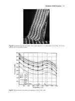
First, we replicate the results from previous studies that found predictability based
on the significance of the predictor variables. As presented in Figure 1 the dividend
yield is significant for almost 60 % of the sample and the change in GDP is significant
for the entire sample. The change in the unemployment rate becomes insignificant
after the first rolling window. The time-varying pattern of the t-values and the co-
Comparison of t-values
t-value
2000 2001 2002 2003 2004
-4
-3
-2
-1

0
1
2
3
4
t-value DivYield
t-value IndPr
t-value UnemplR
Fig. 1. Comparison of t-values of linear regression over time
efficients of the predictors (not reported) are in line with Bessler and Opfer (2004).
Thus, model uncertainty is not a static problem but rather needs to be taken into ac-
count over time as well. A comparison of squared errors over time for the six models
reveals that the AR(1) and the BVAR yield the best results (Figure 2). All models
show a similar pattern with peaks occurring in those months when returns are both
very high in magnitude and negative most of the time. Thus, such extreme returns
cannot be predicted with these models. By taking a closer look at the two models with
the best forecasting performance, i. e. the AR(1) and the BVAR, two issues should
be noted. The difference in squared errors between the AR(1) and the BVAR in the
upper panel of Figure 3 reveals that the BVAR is superior in normal markets. Never-
theless, the AR(1) performs better in down markets. This can be explained with the
increasing (positive) autocorrelation in returns during market turmoil. The change in
autocorrelation is not reflected in the BVAR as its forecasts do not respond to shocks
as quickly as the AR(1) forecasts. However, a comparison of the MSE for the six
models indicates that none of the models produces significantly better forecasts than
a naive forecast.
504 Wolfgang Bessler and Peter Lückoff
Random Walk (# 14)
SE (in ’000)
2000 2001 2002 2003 2004
0

25
50
75
100
125
150
AR(1)-Model (# 13)
SE (in ’000)
2000 2001 2002 2003 2004
0
25
50
75
100
125
150
Box Jenkins (# 10)
SE (in ’000)
2000 2001 2002 2003 2004
0
25
50
75
100
125
150
Linear Regression (# 2)
SE (in ’000)
2000 2001 2002 2003 2004
0

25
50
75
100
125
150
VAR(4)-Model (# 17)
SE (in ’000)
2000 2001 2002 2003 2004
0
25
50
75
100
125
150
BVAR(18)-Model (# 23)
SE (in ’000)
2000 2001 2002 2003 2004
0
25
50
75
100
125
150
Fig. 2. Squared forecasting errors for 1-step ahead forecasts over time
BVAR(18)-Model (# 23) vs. AR(1)-Model (# 13)
SE (in ’000)
2000 2001 2002 2003 2004

-20
0
20
40
60
80
100
AR(1)
BVAR(18)
Diff
Return of Portfolio
Return in %
2000 2001 2002 2003 2004
-360
-270
-180
-90
0
90
180
270
Fig. 3. Comparison of squared forecasting errors for BVAR and random walk
4.2 1- to 15-step forecasts
By looking at longer forecasting horizons of up to 15 months, the dominance of the
BAVR becomes even more pronounced (Figure 4). However, the simple AR(1) still
provides comparable results.
4.3 Single stocks as variables
An interesting result emerges when we substitute the macroeconomic variables in
the BVAR with the return series of the ten stocks of the portfolio. The forecasting
performance of the BVAR based on single stock returns improves significantly. For

example, over a forecasting horizon of 12 months the MSE of the BVAR is about
3 percentage points smaller than the MSE of a naive forecast. The superior results
Predicting Stock Returns with Bayesian Vector Autoregressive Models 505
Random Walk (# 14)
Forecasting horizon
MSE (in ’000)
51015
0
5
10
15
20
25
30
AR(1)-Model (# 13)
Forecasting horizon
MSE (in ’000)
51015
0
5
10
15
20
25
30
Box Jenkins (# 10)
Forecasting horizon
MSE (in ’000)
51015
0

5
10
15
20
25
30
Linear Regression (# 2)
Forecasting horizon
MSE (in ’000)
51015
0
5
10
15
20
25
30
VAR(4)-Model (# 17)
Forecasting horizon
MSE (in ’000)
51015
0
5
10
15
20
25
30
BVAR(18)-Model (# 23)
Forecasting horizon

MSE (in ’000)
51015
0
5
10
15
20
25
30
Fig. 4. Squared forecasting errors for 1- to 15-step ahead forecasts
based on single stocks rather than macroeconomic variables can not be explained
by a decoupling of returns from macroeconomic factors during the rise and fall of
the new economy era. The MSE for the subsample including the downturn up to
03:2003 is only about 1 percentage point smaller than the naive forecast’s MSE over
all forecasting horizons. In contrast, for the subsample from 04:2003 onwards, the
MSE is at least 2 percentage points smaller than that of a naive forecast and again
the lowest for a 12 months horizon (6.5 percentage points smaller) which implies a
high degree of predictability.
5 Conclusion and outlook
The objective of this study was to evaluate the forecasting performance of BVAR
models for stock returns relative to five benchmark models. Our results suggest that
even if we can reproduce the predictability results of earlier studies based on the
significance of parameters none of the models based on macroeconomic variables
is capable of predicting stock returns as measured by forecasting errors. However,
there is a certain degree of predictability of the BVAR when we use the returns of
single stocks instead of macroeconomic variables. Thus, it seems worthwhile to take
a closer look at the cross-correlation structure of stock returns over monthly horizons.
For future studies we suggest to use asymmetric weighting matrices for the prior
that take into account the differences between industries (cyclical vs. non-cyclical)
and sizes of the companies. Alternatively, our methodology could be extended to an

application on bond markets as it is derived from a simple present-value relation.