Student t-test for dependent (matched/paired)
samples
Maintaining variability at as low a level as possible is an important considera-
tion in the design of experiments. One means of mi nimizing variability is to
design an experiment on a paired or matche d basis. Imagine we want to
examine the e⁄cacy of a new ‘long-acting’ formulat ion of aspirin (Z) with a
standard compressed tablet preparation (Y). We could recruit eight patients
who would be willing to participate in the experiment, but there is l ikely to be
many factors that vary within the patient group ^ they are all not going to be
the same height, weight or age, have the same state of health or have symptoms
of exactly the same severity. Wh at rules can we apply to the experimental
conditions to ensure that these factors are minimized?
1. Each patient can have adminis tered, on separate occasions, the new formu-
lation and the standard aspirin preparation. As the assessment of the
e⁄cacy o f the treatment will be carried out by the patients themselves, any
intra-subject variability will be eliminated by generating matched data.
2. Bias may be removed from the experiment by adopting a double-blind
technique. The order in which th e preparations are administered can be
randomized (four patients will re ceive aspirin on the ¢rst occasion, whilst
the remaining four will receive the new drug) and the experiment will be
double-blind. A double-blin d design means that both treatments will be
coded (Yor Z) so that neither the patient receiving the medication nor the
doctor giving the tablets will be able to identify whi ch treatment is being
given. T he code for the treatm ent is kept by a third, independent party.
Section 2.2 discusses study designs to eliminate bias.
At the e nd of the experiment the investigator will have an assessment of the
number of hours of pain rel ief from the patients. In the experiment we have
generated paired data as the subje cts have acted as their own control. The
paired t-tes t can therefore be used to analyse the data.
Exercise 5.3
The results of the experiment can be seen in Table 5.3.

Open a new workbook in Excel and enter the data, as in the
last exercise, in two columns. The assumptions about the test,
121STATISTICAL TESTS FOR TWO SAMPLES
reason for using a paired analysis and hypotheses should be
included on the worksheet. We will be adopting a two-tailed
test as before as we cannot be certain as to whether the new
formulation will increase or bring about a decrease in the hours
of pain relief in the patients.
When this has been completed, from the Data Analysis menu
select t-Test: Paired Two Sample for Means. A dialogue box
should appear similar to that in Figure 5.1. Input the range of
cells for the data for each column under Variable 1 range and
Variable 2 range. Include the rows that have the titles for your
data and tick the check box Labels.
Ensure that Alpha is set at 0.05 and choose where on the
worksheet you would like the results of the analysis to appear.
Click OK to confirm your choices.
The data analysis table in Figure 5.3 should now be shown on
the worksheet.
From the analysis table we can see that there are a few
differences from the previous test results. Firstly, if we were
calculating the t-statistic using the set formula we would need
to subtract individual values in each column from each other as
the analysis uses the differences between pairs. This has
resulted in a negative value being returned for the calculated t-
statistic. We ignore the negative sign, as it is only the numerical
122 5 STATISTICAL ANALYSIS
Table 5.3 Pain relief in eight patients administered standard aspirin tablets and a new dr ug
on two separate occasions as par t of a double-blind study
Patient

Hours of pain relief with
standard formulation (Y)
Hours of relief with
new formulation (Z)
13.23.8
2 1.6 1.8
3 5.7 8.4
4 2.8 3.6
55.55.9
61.23.5
76.17.3
8 2.9 4.8
value that we use (if we had our data organized with the
column of values for Z first on the worksheet, then Y, we would
have a pos itive value for t-Stat, but the numerical value will still
remain as 3.8319).
The calculation of the degrees of freedom is also different.
For the paired t-test the degrees of freedom is equal to the
number of pairs of data minus one, i.e. df ¼871 ¼7.
Comparing the calculated value of the t-statistic with the
critical two-tailed value at the 5 per cent level of significance,
we can see that the calculated value is higher than the
tabulated value (3.83242.364). We can conclude that there
is a significant difference in the hours of pain relief produced by
the new formulation Z compared with the standard aspirin
preparation Y and therefore reject the null hypothesis and
accept the alternative. As before, Excel shows the actual
significance level which is 0.0064 (0.64 per cent). We may
make a full statement about the conclusions of the analysis by
comparing the means and variance of the data as in the first

exercise.
123STATISTICAL TESTS FORTWO SAMPLES
Figure 5.3 Output data for the dependent (paired) t-test
Non-parametric tests for two samples
T hese tests are us ed where we have either ordinal data or interval level data
from populations which are not normally distributed (or their shape is
unknown). When using summary statistics to describe the results from non-
parametric tests is it more appropriate to use median values rather than the
mean (that is used for parametric tests).
. The Wilcoxon signed rank test is used for matched or paired samples.
. The Mann^Whitney U-test is used for independent samples.
Neither of these tests can be performed automatically in Excel through the
Data Analysis options, but making use of the functions on the worksheet the
appropriate statistics can easily be obtained.
The Wilcoxon signed rank test
T he sign test uses in formation on the direction of di¡erences between data in
pairs and, by ranking the d ata, the magnit ude of the di¡erences is also taken
into consideration. We will look at an example where patients su¡ering from
rheumatoid arthritis were asked to grade their joint sti¡ness after one month
of treatment having taken a standard treatment compared wi th a new drug, in
a randomized double-blind stu dy. The patients were asked to record the
degree of sti¡n ess in the a¡ected joints immediately upon waking in the
morning and rate it on a scale between 0 and 5, where 0 indicates no sti¡ness
and 5 represents complete immobility. As the patient’s scores are likely to be
subjective it is important that paired data are obtained and that a non-
parametric test is applied. The Wilcoxon signed rank test is chos en as this is
for matched data.
Exercise 5.4
Enter the data from Table 5.4 in two columns on the Excel
worksheet as in previous tests. State the basis of the test:

Null hypothesis: There is no difference in the scores for joint
stiffness in the patients taking the standard treatment com-
pared with the new drug.
12 4 5 STATISTICAL ANALYSIS
Alternative hypothesis: There is a difference in the scores for
joint stiffness in the patients taking the standard treatment
compared with the new drug.
Level of significance : 5 per cent.
The test is two-tailed as we cannot be certain that the new
compound will improv e joint mobility.
In order to complete the Wilcoxon test you will need to work
through steps 1–6 below.
Step 1
As the data are paired, the first step is to take the differenc e
between each pair. Label a new column next to ‘New drug’
called ‘Difference’.
In the first cell enter a formula to calculate the difference
between the scores for each treatment for patient 1, i.e. if your
first row of data begins in B2, then type in ¼B27C2 and press
Enter. An answer of 0 should now appear in cell D2. Using the
Autofill handle (see section 3.1) copy the formula down the
column to calculate the differences between the remaining
pairs of data. Your worksheet should now appear as in
Figure 5.4.
125STATISTICAL TESTS FORTWO SAMPLES
Table 5.4 Scores recorded for joint sti¡ness in a group of10 pati ents
Patient number Standard treatment New drug
133
241
342

422
501
613
722
812
932
10 3 1
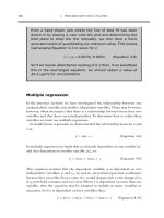
Step 2
Type the title ‘Sign’ in the column next to ‘Difference’. You will
now record the Sign (+ or 7) of the differences. Where a sign is
negative a value of 71 will be entered, where a sign is positive
1 is entered. Click on first cell in the Sign column (cell E2 in
Figure 5.4). From the Paste Function select SIGN and enter the
cell reference (D2). A 0 will appear as there is no sign attached
to a value of 0, but if you use the Autofill handle to copy the sign
function down the column, values will appear in the other cells.
Compare your worksheet with Figure 5.5.
126 5 STATISTICAL ANALYSIS
Figure 5.4 Data table for the Wilcoxon signed rank test
Figure 5.5 Adding signs to theWilcoxon signed rank test
Step 3
We now need to use the difference between each pair, but
remove any negative values, as in the next stage of the
analysis the differences will be ranked. The simplest way to
accomplish this is to multiply the Difference by the Sign to
return positive values for all the differences. Enter the title
‘Sign6difference’ in the next column and in the cell below enter
a formula to multiply the value in the first cell in the Difference
column (D2) by the Sign (0), i.e. in this example ¼D2
*

E2. The
value of 0 should be returned which can then be copied down
into the remaining cells.
Step 4
The next stage is to sort the data so that they may be ranked.
When data from a table is sorted, ALL of the data in the table
has to be selected. If this approach is not taken, then the
sorting process will scramble the data.
Select the data, i.e. all rows and columns containing data on
the worksheet including labels. Using the Datajj Sort command
select Sign6difference from the drop down menu as in Figure 5.6
127STATISTICAL TESTS FORTWO SAMPLES
Figure 5.6 Sorting data for Sign6di¡erence
and sort the data into ascending order. The worksheet should
have the data listed as in Figure 5.7.
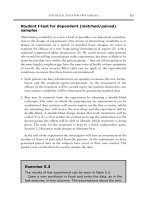
Add the title Rank to the column next to Sign6difference
(G2). The data need to be ranked manually as there are some
rules to be applied when ranking data. Firstly, there are three
values of 0. It is a rule for the test that any zero differences
between the pairs are excluded from the analysis. The ranking
should therefore start with the first (and lowest) value of 1.
However, there are three Sign6difference values of 1. We
therefore have to consider these values as occupying ranking
positions 1, 2 and 3 (N.B. If all of the values were diffe rent then
these would be the ranks assigned.) Because the values are
identical we have to award ‘tied ranks’ to give them equal
weighting in the analysis. A tied rank is the average value of
ranks, so the average of ranks 1, 2 and 3 will be 2. Next to the
three values of 1 enter ranks of 2. We are now ready to
continue ranking. The following values in Sign6difference are

three values of 2. These will occupy ranking positions 4, 5 and
6; as the mean of these is 5 we enter this value in the Rank
column. The last value is 3, so this occupies rank 7.
12 8 5 STATISTICAL ANALYSIS
Figure 5.7 Preparing to rank data for the Wilcoxon signed rank test
Ranking
Both theWilcoxon and the Mann^Whi tney tests use ranked data.
If two or more values are the same in the list to be ranked, give each value
the mean of the ranks they occ upy (as in the example).
Any d i¡ere n ces of 0 should no t be ranke d. You should ignore any ze ro
di¡erences.
Step 5
Now the Signed Rank needs to be calculated. (This indicates
the direction of your data, so brings back the + or À status of
the differences.) Enter the title Signed Rank into cell H1. The
sign of the rank is calculated by multiplying the Sign by the
Rank value (by applying the formula ¼G5
*
E5 in the example
shown). Using the Autofill handle, copy the formula down the
column.
Step 6
In the final step we separate positive ranks from negative ranks
from which we will calculate the totals of each set (the lower of
these two totals will be used as the critical value of T, the
Wilcoxon statistic).
Using Datajj Sort, sort all of the Signed Rank values into
ascending order. This will group all of the positive and negative
values together. Separate positive ranks from negative ranks
and calculate the totals using the AutoSum function. (To do this

you can use the copy button. Select the first cell where you
want the data to appear and then Edit: Paste Special, choosing
Paste Values from the list.) Your worksheet should now have
the totals for each column as shown in Figure 5.8.
If we compare values for the sums of the positive and
negative ranks, the negative ranks total is smaller (9).
Whichever value is the smaller (rega rdless of its sign) is
taken to be the calculated value (T). Now refer to the table of
critical values for the Wilcoxon signed rank test in the
129STATISTICAL TESTS FORTWO SAMPLES
Appendix. If the calculated value for T is smaller than the
critical value then we would reject the null hypothesis. From
the table we can see that the critical value for seven pairs of
data is 2 at the 5 per cent level (note that although there are 10
subjects in the study we exclude any pairs where the difference
was zero). Our calculated value is greater than the critical
value, therefore, we reject the alternative hypothesis and
accept the null hypothesis for the experiment. We can conclude
that there is no apparent difference perceived by the patients in
relieving the symptoms of morning stiffne ss by the new drug.
The Mann^Whitney
U
test
T he Mann^Whitney tes t is th e non-parametric te st used for independent data,
and may be conducted with unequal or equal sample sizes. I n the example
given here, sample sizes are unequal, but procedures are exactly the same for
equal sample sizes.
Exercise 5.5
A team of investigators wanted to investigate the claim that a
particular technique could be used to improve memory. They

took two groups of subjects of similar ages and educational
130 5 STATISTICAL ANALYSIS
Figure 5.8 Separating positive and negative ranks
ability and subjected each group to a test in which they were
given a list of 50 items on a list to memo rize. One group was
provided with a 1-hour session before the test in which they
were given training in the technique. The data from the
experiment are listed in Table 5.5.
Null hypothesis: Training in a memory technique does not
have any effect on the ability of subjects to recall a list of 50
items.
Alternative hypothesis: Training in a memory technique does
have the effect of improving the ability of subjects to recall a
list of items.
Level of significance : 2.5 per cent.
A one-tailed test is used as the researchers have predicted the
direction of the outcome (i.e. the memory of the test subjects
could not have been impaired by the training technique).
131STATISTICAL TESTS FORTWO SAMPLES
Table 5.5 Number of words recalled by two groups of subjects, one of
which was given training in the application of a memory technique
Control group Treated group
26 15
14 45
32 44
25 41
19 25
15 37
31 42
33 26

29 36
26 14
37 27
29 44
23 41
30 26
28
33
We will now apply the Mann–Whitney non-parametric test for
independent variables to the test data.
Step 1
Open a new worksheet in Excel. Enter the data from Table 5.5
onto your worksheet, but place it in two columns as shown in
Figure 5.9 so that in the first column a code is applied to
indicate whether the subject’s data belong in the control (c)
group or the trained (t) group.
Step 2
The data now needs to be ranked applying the same principles
as the Wilcoxon test; but first we must sort the data. Highlight
the cells containing the data and then select DatajjSort. Sort
Items Recalled in Ascending order. Enter Rank into the cell next
to Items Recalled. Now give a numerical rank to all of the data,
keeping in mind that if values are identical, the mean rank
should be entered.
Step 3
The two data sets are separated into control and treated groups
once more. To do this we perform another sort, this time
selecting to sort the Group alphabetically (select all cells
containing data on the worksheet and sort using the Alphabe-
tical Sort button on the toolbar). The two data sets now need to

be separated.
Select the data for the treated subjects (n ¼16) and copy and
move the tr eated data as a block into the three columns
adjacent to the control values as shown in Figure 5.10.
(Highlight the three columns to be moved and drag on the
border to achieve this.)
Using the AutoSum button calculate the sum of ranks for
both control and treated groups.
Step 4
Using the sum of ranks we can calculate the value of U (the
Mann–Whitney statistic) from the formula:
132 5 STATISTICAL ANALYSIS
U ¼ n
1
n
2
þ n
1
ðn
1
þ 1Þ
2
À R (Equation 5:1Þ
where n
1
is the number in the smalle st sample
n
2
is the number in the largest sample
R is the sum of ranks of the smaller data set

This formula can be placed into a cell on the worksheet.
¼ð14 Ã16Þþð14 Ãð14 þ1Þ=2ÞÀ173:5
133STATISTICAL TESTS FORTWO SAMPLES
Figure 5.9 Data for the Mann^Whitney test
On pressing the Enter key a value of 155.5 for U should be
returned.
Step 5
In order to complete the test we need to calculate the value for
U’ using the formula:
U’ ¼ n
1
n
2
À U (Equation 5:2Þ
Enter the formula, ð14 Ã 16ÞÀ155:5, into an empty cell. The
value of 68.5 should be returned for U’.
Of the two values, U and U’, we take whichever is the smaller.
In this example U’ is smaller with a value of 68.5.
We now need to look up the critical value of U using the
Mann–Whitney U tables in the Appendix, using n
1
and n
2
. The
null hypothesis is rejected and the alternative accepted where
the smaller value of U or U’ (whichever applies) is less than or
equal to the critical value of U. As the critical value U is 64 we
can reject the alternative hypothesis and accept the null
hypothesis (the calculated value of U’ is greater than the
134 5 STATISTICAL ANALYSIS

Figure 5.10 Totalling the rank data for the control and treated groups
critical value). The memory training clearly did not have any
effect on the number of items recalled by the subjects (median
for the control group is 29 items; median for the trained
subjects is 34.5 items).
N.B. Both non-parametric tests, the Wilcoxon signed- rank test and
Mann^Whitney U-test, rely on the calculated value being smaller than
the crit ical valu e to demonstrate signi¢cance.
5.3 Analysis of variance
In the previous section we h ave considered how to test data when we have two
samples. Quite frequently though, we design an experiment in which we make
multiple comparisons as there are several treatments or conditions applied that
we want to compare with a control. Including more than one treatment
minimizes any variation that might be encountered by conducting several
smaller expe riments or investigations over a long er period of tim e, such as
seasonal variations, di¡erences in batches of reag ents etc., not to mention the
cost and resource implications.
As part of designing an experiment where a number of di¡erent treatments
are applied, an appropriate statistical test ne eds to be considered at the
planning stage. This is particularly important where the experiment is quite
complex to ensure that a ‘balanced’ design is achieved. In balancing an
experiment we ensure that there will be either equal replication into grou ps
(known as blo cks) or treatments, or that there will be equal precision in the
comparison of variables that are investigated.When an experiment is properly
balanced we can expect to apply the simplest s tatist ical analysis from which to
demonstrate our conclusio ns with clarity and unambiguity.
Let us th ink through an experiment in which we want to investigate the
e¡ects of several di ¡erent concentrations of a growth hormone on the grow th
of plant sections. To conduct a fair test we need to include a control in which
the media used for containing the plants would not have any growth hormone

present. Then, instead of designing a seri es of experim ents in which a single
concentration of hormone would be investigated agai nst a control, we would
design an experiment in which several di¡erent concentrations we re compared
simultaneously. So we may have a design in which we have:
135ANALYSIS OF VA RIANCE
Treatment
Control A B C D
in which treatments A^D would each represent a di¡erent concentration of
hormone. Having completed the experiment you might then be tempted to use
a Student t-test to compare the growth of plant sections grown in the control
media with each individual treatment in turn. Th is would be incorrect, unless
special conditions we re applied, and in statistical terms is known as mak ing a
Type I error. This is because we would need to make several analyses to be able
to compare all of the data to know whether a di¡erence exists between the
control an d di¡erent concentrations, and also whether the concentration itself
contributes to the extent that the plan t section grows. In order to make a full
set of comparisons we would need to perform t-tests as follows:
ControlvsA AvsB BvsC CvsD
ControlvsB AvsC BvsD
ControlvsC AvsD
Control vs D
T his would mean performing 1 0 tests in total. It may be di⁄cult to understand
why it would b e wrong to make this number of comparisons. The answer is
that we might falsely conclude that there is a signi¢cant di¡erence between
treatments as a consequence of performing so many statistical tests, and not
on account of any real di¡erence in the data. When we form the basis of a
statistical test we formulate hypotheses and set a level of signi¢cance, usually
at 5 p er cent. This means that we are accepting the probability of an event
occurring by chance alone is 5 per cent or less.To try to visualize the problem,
let us think of a the probability in a statistic al test as being a box containing

100 balls. Five of the balls will be red; the remaining 95 white. If we remove a
ball from the box (in conducting the test) then there is a chance of 5 per cen t
that the ball will be red. If the ball that is removed is white and we then remove
another ball (testing the data again) then there is an increas ed likelih ood of
obtaining a red ball (5 out of 99). This situati on is analogo us to performing
two tests on the same data set. So in our situation, where 10 comparisons need
to be made, the p ossibility of demonstrating a false signi¢cant di¡erence
would increase each time the test is performed. A Type I error is therefore a
situation in which we wrongly assume that there is a di¡erence between
samples and incorrectly reject the null hypothesis.
There are two ways in which we could obviate this happening. The ¢rst
would be to lower the level of signi¢cance, min imizing the opportunity of a
false positive result; but then we may commit aType II error as a real signi¢cant
136 5 STATISTICAL ANALYSIS
di¡erence may be missed. The second option is to use an analysis of variance
(ANOVA) test which removes any possibility of a Type I error as the data is
tested all together; this opti on is preferred as the ANOVA is also a more
powerful stati stical test in this situation. The power of a test is de¢ned by its
ability to correctly reject the null hypothesis under the conditions set.
T he analysis of variance uses all of the data and retur ns a single probability
value. Should this show that there is a signi¢cant di¡erence between treat-
ments in the data set then furthe r analysis, in the form of a multiple range tes t
has to be performed. According to the design of the invest igation, eithe r a one-
way (for one-factor comparisons) or a two-way (for two-factor comparisons)
ANOVA tes t can be applied. In th e followin g su bsect ions we will look at
examples of each of these tests and demonstrate how a multiple range test can
be applied.
One-way analysis of variance
This analysis is ap plied for one-factor comparisons; so for the comparison of
the growth of the plant sections, the only factor investigated was hormone

concentration. In this situation a one-way analysis would be suitable. However,
we will take as our example to work through in Excel an experiment in which
the e¡ect of pH on drug dissolut ion was investi gated. A preparation of aspirin
containing 100 mg of drug was placed in solutions of di¡erent pH for a period
of 12 hours in a rotating basket. Samples from each solution we re taken at
periodic intervals and at the end of the experiment the amount of drug that
had dissolve d was calculated. The exp eriment was repeated ¢ve times at each
pH. The purpose o f the experiment was to examine wh ether the pH of the
dissolution med ium had any e¡ect on drug dissolution and if s o, to in d icate at
which pH optimum dissolution occurred.
Exercise 5.6
Enter the data in Figure 5.11 on the Excel worksheet as shown.
Before commencing the test, the null and alternative
hypotheses need to be stated, together with the level of
significance to be adopted:
Null hypothesis: There is no difference in the dissolution of the
aspirin tablets in different pH solutions.
137ANALYSIS OF VA RIANCE
Alternative hypothesis: There is a difference in the dissolution
of aspirin when expos ed to different pH solutions.
Level of significance: 5 per cent (P50.05).
Using the ToolsjjData Analysis function, select the ANOVA:
Single Factor (this is the one-way analysis of variance) option
from the menu. As shown in Figure 5.12, enter the range of
values for the cells containing the data and check the box for
the labels so that the pH will be displayed in the resu lts of the
analysis. Our data is in columns, so ensure that this is also
checked on the dialogue box before clicking OK.
The analysis for the data will now appear on the worksheet,
as shown in Figure 5.13. Excel produces the mean and variance

for each set of results at different pH values. From the ANOVA
table the value of F can be seen to be 1676.2, greatly in excess
of the Critical value of F at the 5 per cent level of significance
(3.2). As in the other statistical tests that we have use d so far,
138 5 STATISTICAL ANALYSIS
Figure 5.11 Inputting data for the on e-way analysis of variance
statistical tables do not need to be used as the P value is
automatically calculated; on this occasion it is 3.41610
720
(shown as 3.41E-20), i.e. P ¼0.000 000 000 000 000 000 03.
This demonstrates that there is a highly significant difference
between the dissolution of the drug at different pH, so we can
therefore reject the null hypothesis and accept the alternative
hypothesis. The problem now arises in deciding how the pH
treatments differ; there are six comparisons to make in total
and we have already indicated that we cannot do a pairwise
comparison using the t-test. How do we test for differences
without increasing the likelihood of a Type I error? The answer
is to use a multiple range test. There are a number of different
types: Tukey, Scheffe´ and least significant difference (LSD)
between means test. They all work in the same way; it is only
the situations in which they are applied that differ slightly. We
will apply a LSD between means test to the data to determine
what differences lie in dissolution rates at each pH. This test
may only be applied where there is an equal number of sampl es
in each treatment.
139ANALYSIS OF VARIANCE
Figure 5.12 Showing the data range for the one-way ANOVA