Data Analysis and Presentation Skills Part 4 ppsx
Bạn đang xem bản rút gọn của tài liệu. Xem và tải ngay bản đầy đủ của tài liệu tại đây (823.9 KB, 19 trang )
In Ste p 2 of 4 you will now see the preview of the chart. (N.B. by clicking on
the Series tab you can edit the chart, adding or removing data that you would
like plotted.) Click Next4 to con tinu e.
In Step 3 of 4 you may add titles and lab els to your graph (see Figure 3.8).
45AN I NTRODUCTION TO MICROSOFT EXCEL
Figure 3.7 Fi rst Step in Chart Wizard showing previ ew of plot
Figure 3.8 Step 3 of Chart Wizard for inputting titles and lab els
In the Chart title box type ‘Species of butter£ie s at Parad ise Common’. In the
Value Yaxis type ‘number observed’. Click on Next4.
In Step 4 of 4 you have the option of eithe r plac ing the chart on a new sheet
or embedding it on yo ur present data sheet. Clic k on ‘As object in’ and then
click Finish.
Your chart will now appear on your datasheet together with a toolbar from
which you may edit the graph. If the toolbar does not automatically appear
then it can be called up by clicking on View, then Toolbars and selectin g Chart
from the list available (see Figure 3.9).You need to click on the graph to select it
for the bu ttons on the toolbar to function.
Try changing the graph from being plotted ‘by column’ to ‘by row’ by
clicking on the appropriate button located towards the right of the toolbar (see
Figure 3.10) .
Individual components of the chart can b e edited using the selections from
the menu on the left-hand side of the dialogue box. For instance the size of the
chart can be adjusted by selecting ‘Plot Area’ from the drop down menu on the
le ft-hand si de of the dialogue box. You can change the dimensions by clicking
on one of the black handles that appe ar on the border and dragging the ch art
to the size that is required.
46 3 PRESENTING SCIENTIFIC DATA
Figure 3.9 Inserting the Chart Toolbar
Changing colours and patt erns in the chart
Click on‘Series April’ from the drop down menu on the toolbar.You should s ee
that all of the bars relating to April have been selected on the plot (a coloured
square appears on each bar ). Now click on the Format Data Series button to the
right of the drop down menu (see Figure 3.11).The colour palette appears from
which a di¡erent colour can be selected.
Now click on the ‘Fill e¡ects’ button beneath the palette and select a ¢ll
pattern of you r choice. Once you have made your selection, click OK. The
Format Data Series option may be used to edit other features of the graph, but
this will be further explained in secti on 3.2.
Gridlines
Gridlines in a chart help to iden tify values for columns; but they are not always
wanted in a chart. Click on one of the gridl ines on your graph; o nce selected,
click the right mouse button. Options appear to format the gridlines; or else ,
by selecting Clear, the gri dlines will be completely removed from the plot. By
47AN INTRODUCTION TO MICROSOFT EXCEL
Figure 3.10 Editin g the graph using the Chart Toolbar
opting for Format Gridlines you are able to adjust the style, weight and colour
of the gridlines.
Adding more data to a chart
More data can easily be added to a chart.
Select cells F4 to F8 which contain the mean data on the worksh eet. Point
on the selected area’s borde r (the mouse pointer appears as an arrow). Drag
over to the chart and release the mouse button (this is known as the ‘Drag and
drop’ method). The new (mean) data will be automatically entered into the
chart.
Note : the last procedure can be undone by clicking on Edit and selecting
Undo Drag and Drop from the menu.
48 3 PRESENTING SCIENTIFIC DATA
Figure 3.11 Selecting colours and patterns from the Format Data Series options
Customizing worksheets
If you are working with a large set of data it is preferable to place data and
analyses o n di¡erent worksheets within a workbook in the same way that data
would be kept on shee ts organized within a folder. To identify the location o f
items within the workbook the tabs on the worksheet can be relabelled. On the
worksheet with the butte r£y data, cli ck on th e Sheet 1 tab once with the right
mouse button. Th is should give you a numb e r of options for the worksheet
such as inserting, deleting, renaming, selecting or moving and copyi ng a sheet.
Select the option to rename the shee t and type butter£ies on the tab, pressing
the Return key to complete the renamin g.
When worksheets are printed out the tab ke ys will not be present, so it
use ful to further customize the sheet so that its contents are clearly marked.
From the File menu select Page Setup (Figure 3.1 2). A number of options
appear that will allow you to change the orientation of the page and print
quality, alter the page margins, insert a header and footer and the character-
istics of the worksheet.We are going to add a customized header and footer, so
select this tab. A number of di¡erent options may be selected to present the
header and footer of each page. As an example we will customize the footer of
thepage(seeFigure3.13).
In the Header lis t box, select None and click on the Custom Footer option.
Three boxes appear that represent the left, centre and right sections of the
page. Start in the box on the left-hand side and type in a ¢lename for your
49AN INTRODUCTION TO MICROSOFT EXCEL
Figure 3.12 Options for the Page Setup
workbook, e.g. butter£ies.xls. It is always useful to have the ¢lename recorded
on a prin ted piece of work to make ¢n di ng the ¢le again mu ch easier should
you want to edit the informatio n in the ¢le. I n the centre section type in your
own name, particularly useful if you are submitting the printed item as
coursework as the worksheet is clearly ident i¢ed as belonging to you. In the
box on the right-hand side we can insert (by cl icking the appropriate option
above) the time and date. Each time the worksheet is opened and saved, the
current date an d time will be recorded on the worksheet.When ¢les are being
updated by adding further information from an experiment or study, it is
important to keep track of when revisions are made, so adding the date and
time aids this process. Con ¢rm the changes that you have just made (by
clicking OK). On retur ning to your worksheet, you should be able to see the
footer by clicking on the Print Preview button. You may alter the properties of
the worksheet by re-entering the Page Setup menu from the top of the page.
Select this option now and we will further adjust the appearance of the
worksheet prior to printing. Choose the options to show the gridline s of the
worksheet and to print in black and wh ite by checking (click on the box so that
an x appears) the appropriate box accordingly.
50 3 PRESENTING SCIENTIFIC DATA
Figure 3.13 Customizing worksheets
Producing tables in Excel
If the information we are usin g in the spreadsheet needs to be used as a table in
a re port, the format ought to be more attractive. The butter£y data can be
formatted into a table (see Figure 3.14). Click on any cell in the l ist of data
en tered on the worksheet, e.g. click on cell C5. From the Format menu on the
toolbar, select Autoformat.
T he ran ge of values around cell C5 will automatically be selected and can be
arranged in one of several pre-set formats. From the Table Format box, scroll
down the options and choose a pre-set format (e.g. Simple1) and clic k OK.The
data are now displayed as a table in the format s elected; the format may be
revised as many times as you like until a satisfactory choice is made. Once you
have completed your revisions, use the Pr int Preview option again to check that
all of the items on the worksheet are going to appear in the correct position on
the page, altering them if neces sary by selecting and mov ing them.This cannot
be done while in Print Preview mode; you will need to return to the worksheet
to do this. After Print Preview has bee n use d you should no tice that the limits
of the page can been seen as dotted lines on the worksheet. Items may then be
moved around by selecting and dragging to format the worksheet within these
borders, ready for printing. Having checked the worksheet thoroughly
(including spellings using Tools:Spelling option) the workbook can be saved
and printed.
3.2 Presenting graphs and charts
Having worked through the previous section you should now realize how
simple it is to produce graphs in Excel. What is more skilful, however, is to
decide the best plot for the type of data being presented. In whatever branch of
science we are involved, observations are made during which we gather data.
51PRESENTING GRAPHS AND CH ARTS
Figure 3.14 Formatting tables
Data can be in various forms; it can be qualitative or quant itative. Qualitative
data ten ds to be descriptive, such as whether an individual is male or female;
alive or d ead; blonde, brunette, grey, etc. Quan titative data is numerical and
measured with precision; for example, an individual may have a height of
173 cm and body mass of 72.3 kg.
During the course of experimen ts we generally collect information from our
investigations (raw data) and apply the following three processes:
. organize the data; e.g. sort into groups, set into a table.
. illustrate the data in order to interpret the information from the investi-
gation; i.e. make into a bar chart, line graph, pie chart.
. analyse the data using an appropriate statistical method; from the statis-
tical test a conclusion may be drawn about the investigation.
We will be thinking about the statistical analysis of data in later sections,
but for now we will look at di¡erent types of data and see how it should be
presented.
Graphs and charts
Drawing a graph in Excel is easy, but does the ¢ni shed item look right? Is it
presented as it should be? Unless you choose the correct type of plot, produ-
cing a graph can go very badly wrong and data can be misrepresented under
these circ umstances. Let us begin by lookin g at a simple absorption spectrum.
Exercise 3.2
In a laboratory experiment the absorption for phenolphthalein,
a pink-coloured indicator, was determined at a range of
wavelengths. Owing to its colouration the optimum absorbance
is likely to lie somewhere in the region of 540 and 560 nm, so
more frequent measure ments were taken within this range,
although the full range of wavelengths investigated was from
450 to 650 nm. Table 3.2 shows the data obtained from the
experiment. Firstly we must decide what type of graph is
appropriate to draw. Where data show a trend with one item of
information being related to the next in a series, i.e. they
52 3 PRESENTING SCIENTIFIC DATA
appear in a speci fic order, then a line graph will show the
relationship between points.
Enter the data onto a worksheet in Excel and then using
Chart Wizard select the option for a Line plot (see Figure 3.15).
Several types of line plots are shown for you to select the most
appropriate. Choose the one described as Line with Markers at
each Data Value (i.e. the one showing points and lines). Onc e
this is selected you will see that the plot is displayed for the
data, but wavelength is incorrectly plotted on the graph instead
of being used as the scale on the x-axis (see Figure 3.16). Th is
is easily amended by click ing on the Series tab and, using the
Remove button, highlight the wavelength label to delete this
53PRESENTING GRAPHS AND CH ARTS
Ta b l e 3. 2 Absorption spectrum for phenolphthalein between 450 and 650 nm
Wavelength
(nm)
450 5 00 520 530 540 550 555 560 570 580 590 600 650
Absorbance 0.2 0.51 0.60 0.65 0.68 0.72 0.73 0.73 0.67 0.63 0.59 0.49 0.31
Figure 3.15 Selecting line plots
data. Then click in the Category x-labels box, select the
wavelength values and you will then see the graph being
replotted with the wavelengths on the x-axis (see Figure 3.17).
At this point look carefully at the graph – can you see
anything wrong with the plot? (See Figure 3.18.) If you can’t,
try looking at the x-axis and then think carefully about how you
would plot these data if you were doing the graph by hand. You
should then notice that the scale is not linear as it should be.
Excel has plotted the data as though each wavelength reading
is equally spaced apart, which is clearly incorrect. So what
action must be taken to remedy this plot? Use the Back button
to take the steps back to the screen where you were able to
select the type of chart that you wanted. Now click on the X:Y
Scatter option as seen in Figure 3.15. This should display the
chart where the scale on the x-axis is now equally divided (see
Figure 3.19).
Continue through to the next step and add a title and labels
to the graph. Once this has been completed, move through to
the next step and then Finish. The graph shown in
54 3 PRESENTING SCIENTIFIC DATA
Figure 3.16 Previewing line plots
55PRESENTING GRAPHS AND CHARTS
Figure 3.18 Completed graph inserted into the worksheet
Figure 3.17 Changing data automatically plotted on graphs
Figure 3.20 should now be what you see on your screen, but
although the plot is correct, there are still a few problems. The
major problem still lies with the arrangement of the scale on
the x-axis. If this was plotted by hand then the axis would not
begin at 0 and end at 800 nm, so this needs to be narrowed to
prevent the data points being lost in the plot window as at
present. This means that it is necessary to edit the graph,
something that is done very easily in Excel, as just clicking on
the graph will automatically take you into Edit mode. The
important thing to remember here is to click at the point on the
graph that you want to edit which can be any item including
lines, points, background, border and gridlines. As we want to
edit the x-axis, click on the graph near the x-axis and then click
once with the right mouse button. As long as you haven’t
selected the entire plot area then you should now see an
option to format the x-axis.
56 3 PRESENTING SCIENTIFIC DATA
Figure 3.19 Changing plots from Line to XYScatte r
From the menu, click on the tab for Scale and then change the
default values for the minimum and maximum values to 400
and 700, with major and minor units of 50 and 10 respectively
(to determine the increments of the x-axis scale). The axis
should now be adjusted as shown in Figure 3.21.
57PRESENTING GRAPHS AND CH ARTS
Figure 3.21 Changing the scale of the x-ax is
Figure 3.20 XY Scatter plot inserted into the worksheet
The plot is now presented as it should be, but there is
duplicated information on the graph. We have labelled the y-
axis as absorbance, but as part of the automatic processes
used in producing graphs Excel has provided a legend (Abs) on
the plot. If we needed to have a legend, then it ce rtainly
shouldn’t be in this abbreviated form; to remove the legend
select it on the graph, click with the right mouse button and
choose Clear from the options.
Editing plots in Excel
T he way that we present our data is a signi¢can t aspect of scienti¢c reportin g
and the importan ce of taking time to experiment with di¡erent styles in which
to por tray ou r data should not b e u nd e r valued.
Remember: charts should be pre s e n ted in order to e ncou rage the reader to
make comparisons and then analyse them. The designer of the chart should
ensure that the data are presen ted in a clear and unambiguous man n e r so as
not to mislead or bias the reader.
Creating a good chart usually means ensuring it is as simple and clear as
possible, so that its message is immediately apparent. Excel allows you to
readily acces s a range of di¡erent chart styles; the problem is deciding which
one to choose for presenting your information.
Bar charts
Bar charts are the sim plest form of chart. They can be used to show numbers,
proportions or ratios. In Excel, th e bar charts are available as bars or columns.
For the Column chart all of the bars are po sitioned vertically and for the Bar
chart, bars are positioned horizontally across the plot. In Exercise 3.3 we will
explore how to use bar charts e¡ectively to present data whe re we are
comparing one or more variables in an experiment.
Exercise 3.3
Copy the information in Table 3.3 onto your spreadsheet. The
data presents the mean weight loss (in kg) of human subjects
who volunteer ed for a trial in which they were asked to follow
58 3 PRESENTING SCIENTIFIC DATA
three different diets (A, B and C), together with the standard
deviations (SD). The data may be compared between male and
female subjects. You should now be familiar enough with the
Chart Wizard function to plot a column chart of this informa-
tion; if you are unsure of what to do then refer back to the
instructions for producing the column chart for the butterfly
data in section 3.1. Clearly, in this exercise we want to be able
to compare the weight loss produced by each of the three diets,
but we also want to compare the comparative weight loss by
each of the two sexes. In our bar chart we need to select an
option where we are able to make a side by side comparison of
males and females on each diet. Select the data for the males
and females, including the labels (but excluding the standard
deviation data) and choose Clustered Columns from the Chart
Wizard options. Label and title the graph appropriately. You
should then have a plot similar to that shown in Figure 3.22.
59PRESENTING GRAPHS AND CHARTS
Table 3.3 Mean we ight loss ( kg) dur ing six months of human su bjects on three di¡erent
dietary regimes: A, B and C
Diet Males Females SD (M) SD (F)
A1192.31.9
B 21 18 3.6 3.1
C 13 14 2.0 1.9
Figure 3.22 Clustered column chart
Displaying values on charts and graphs
Sometimes it is helpful to show the numerical values for plotted variables on
the graph. To insert values for each column in the plot, click on the chart to
enter edit mode. Select one of the bars in the chart representing data for the
male su bjects (place the mouse pointer over the bar and click), then right click
with the mouse button. From the menu choose Format Data Seri es and then
select the Data L abels tab. You then have the o ption to show the value or show
the label. Choosing Show Value will result in the value being displaye d over all
of the bars in the series that you have selected. The process will need to be
repeated for the bars representing female subjects.
Error bars
In scienti¢c data where a mean value has been calculated, we frequently want
to show the variability of the data by insert ing error bars to represent standard
deviation or standard error (the standard deviation and standard error are
discussed in Section 4). In a bar or column chart the bars need to be inserted at
the top of the bar as shown in Figure 3.23.
Enter edit mode by clicking on the chart and go to Format Data Series as
described above to show the numerical values. Select the tab for Y Error Bars.
60 3 PRESENTING SCIENTIFIC DATA
Figure 3.23 Inserting error bars
Di¡erent opti ons are shown for the types of error bars available. Clearly for a
bar series we n eed the Plus type, so click on this option. Below this you are
prompted to i n dicate how the error value should b e derived. To input a SD or
SE based on data on the worksheet , go to the Custom box. In the + box, type in
the cell references for the cells containing the s tandard deviations for the bars
that you have selected (either the male or the female subjects). Con¢rm the
selection by clicking OK. The chart should now b e up dated with error bars,
but the process will have to be repeated for the second data series.
Finishing touches
It is important to ensure that all graphs are appropriately labelled and titled.
Here are some hints and tips to follow to make sure that plo ts are properly
presented.
1. Axes should have lab els that explain the variables and g ive the un its of
measurement normally by providing the standard scienti¢c abbreviation for
the units in brackets, so‘kilogm’ for kilograms would be unacceptable, but
‘kg’ is correct. Note that some units are arbitrary, as in Exercise 3.2 where
absorbance of phenolphthalein was measured; absorbance does not have
units.
2. Symbols for units in graphs can be inserted into plots using a code for each
symbol. Quite frequently we need to insert symbols such as 8C for degrees
Celsius or mg for micrograms. Symbols have unique codes that can be
en tered by pressing the ALT key and the appropriate numeric code on the
number pad (N.B. it must be using the number pad otherwise this feature
will not work). For example m will be inserted by pressing ALT then 0181. A
list of us e ful code s is provided i n the Appe n d i x.
3. Title s of graphs should be short and concise. The chart title should be clear
about:
. The group or sample that is being described (subjects, male and female).
. The variables involved (diet A, B, and C).
. The type of data presente d (weight loss (kg)).
In sc ienti¢c investigations we frequently per form experiments or trials and
there is a tendency to start titles by writing ‘An experiment to show . . .’or ‘An
investigatio n of . . .’. It is not necessary to start a title in this fashion and it is a
61PRES ENTING GRAPHS AND CHARTS
prac tice that should be avoided. Titles are more readable if the important
information is placed ¢rst, for example,
‘Mean weight loss in male and female subjects
following diets A, B and C (mean+SD)’.
as opposed to:
‘An investigation of the mean (+SD) weight loss in male and female
subjects following three di¡erent dietary regimes (A, B and C)’.
Clearly the ¢rst title is su ccinct and provide s the message of the graph very
clearly.
Framing and gridlines
Most charts bene¢t from having a frame, especially if they contai n gridlines.
E xcel has the facility to change the background of a chart to di¡erent colours.
A light shading is preferred so that it does not interfere with the emphasis of
the chart. Some caution needs to be used wh en printing in black and white as
even what appears as a pale grey background can spoil the appearance of the
chart, particularly where a contrast is needed between the colum ns on the
chart and the background colour.
Gridlines make most charts easier to read as they provide references for us
to judge the values of bars or points. In very simple charts, however, they can
prove to be a distraction and are better removed.The formatting of gridlines is
als o important as they need to be as unobtrusive as possible. They should be
spaced at appropriate intervals. Too many will make the chart appear busy;
whereas too few will not provid e su⁄c ient reference poin ts.
Formatting gridlines
Click on a grid line, then right click the mous e button. Select options under
Style and Weight to reformat the gridlines.
Setting the correct proportions for the chart
Sometimes when a chart is placed directly onto the worksheet it appears as a
small and narrow plot, as shown in Figure 3.24. You should e nsure that the
62 3 PRESENTING SCIENTIFIC DATA
¢n ished item does not look li ke a widescree n TV, by re-prop ortion i n g the
graph and adjust ing the size of the font for titles and labels when necessary.
There is sometimes a tendency to accept whatever the software produces
without questioning whether the mes sage is clearly co nveyed in the graph or
whether extra work needs to be do ne to adjust some of the components of the
plot. The editing features of Excel are very easy to use and there is no excuse
for presenting substandard plots and blaming it on the software.
Exploring different types of bar charts
Stacked column bar ch arts
This is a slightly di¡erent way in which we are able to convey information and
the message of the graph might be di¡ere nt from the graph where bars are
positio ned side by si de. It is useful for summarizing what has occurred in an
investigatio n, but allows us to see data from subgroups and therefore assess
the contribution of components within the experiment. The mean data for the
diets could be represen ted in this way if, for instance, we were interested in
comparing the total mean weight loss between male and female subjects, but
wanted to see the individual contribution of each diet to the weight loss as a
whole. Using the Chart Wizard function, re- plot the data selecting the Column
chart option with stacked columns. As you produce the graph you must ensure
on Step 2 that you change the Series opti on so that the data are organized in
rows instead of columns. This will produce the si de by side comparison o f the
mean weight loss for males and females.Your graph should appear as in Figure
3.25.We can see from this graph that the mean weight loss was greater in the
male than in the female subjects; whereas in our previous graph, Fig ure 3.22,
the emphasis was on comparing the weight loss between diets and showing
that Diet B produced the largest weight loss. If you have plotted the graph and
it appears exactly as in Figure 3.25 you may want to consider how the appear-
ance of th e plot could be made clearer.The legend, for instance, shows Diet A,
63PRESENTING GRAPHS AND CH ARTS
Figure 3.24 Example of a graph that needs re-sizing