Fundamentals of Corporate Finance Phần 7 pot
Bạn đang xem bản rút gọn của tài liệu. Xem và tải ngay bản đầy đủ của tài liệu tại đây (388.66 KB, 66 trang )
386 SECTION FOUR
inflation rate of 3 percent. The firm believes that it will remain in the building for 4
years. What is the present value of its rental costs if the discount rate is 10 percent?
The present value can be obtained by discounting the nominal cash flows at the 10
percent discount rate as follows:
Present Value at
Year Cash Flow 10% Discount Rate
1 8,000 8,000/1.10 = 7,272.73
2 8,000 × 1.03 = 8,240 8,240/1.10
2
= 6,809.92
3 8,000 × 1.03
2
= 8,487.20 8,487.20/1.10
3
= 6,376.56
4 8,000 × 1.03
3
= 8,741.82 8,741.82/1.10
4
= 5,970.78
$26,429.99
Alternatively, the real discount rate can be calculated as 1.10/1.03 – 1 = .067961 =
6.7961%. The present value of the cash flows can also be computed by discounting the
real cash flows at the real discount rate as follows:
Present Value at
Year Real Cash Flow 6.7961% Discount Rate
1 8,000/1.03 = 7,766.99 7,766.99/1.067961 = 7,272.73
2 8,240/1.03
2
= 7,766.99 7,766.99/1.067961
2
= 6,809.92
3 8,487.20/1.03
3
= 7,766.99 7,766.99/1.067961
3
= 6,376.56
4 8,741.82/1.03
4
= 7,766.99 7,766.99/1.067961
4
= 5,970.78
$26,429.99
Notice the real cash flow is a constant, since the lease payment increases at the rate of
inflation. The present value of each cash flow is the same regardless of the method used
to discount. The sum of the present values is, of course, also identical.
᭤
Self-Test 3 Nasty Industries is closing down an outmoded factory and throwing all of its workers
out on the street. Nasty’s CEO, Cruella DeLuxe, is enraged to learn that it must con-
tinue to pay for workers’ health insurance for 4 years. The cost per worker next year will
be $2,400 per year, but the inflation rate is 4 percent, and health costs have been in-
creasing at three percentage points faster than inflation. What is the present value of this
obligation? The (nominal) discount rate is 10 percent.
Separate Investment
and Financing Decisions
When we calculate the cash flows from a project, we ignore how that project is financed.
The company may decide to finance partly by debt but, even if it did, we would neither
subtract the debt proceeds from the required investment nor recognize the interest and
principal payments as cash outflows. Regardless of the actual financing, we should view
the project as if it were all equity-financed, treating all cash outflows required for the
project as coming from stockholders and all cash inflows as going to them.
Using Discounted Cash-Flow Analysis to Make Investment Decisions 387
We do this to separate the analysis of the investment decision from the financing de-
cision. We first measure whether the project has a positive net present value, assuming
all-equity financing. Then we can undertake a separate analysis of the financing deci-
sion. We discuss financing decisions later.
Calculating Cash Flow
A project cash flow is the sum of three components: investment in fixed assets such as
plant and equipment, investment in working capital, and cash flow from operations:
Total cash flow = cash flow from investment in plant and equipment
+ cash flow from investments in working capital
+ cash flow from operations
Let’s examine each of these in turn.
CAPITAL INVESTMENT
To get a project off the ground, a company will typically need to make considerable up-
front investments in plant, equipment, research, marketing, and so on. For example,
Gillette spent about $750 million to develop and build the production line for its Mach3
razor cartridge and an additional $300 million in its initial marketing campaign, largely
before a single razor was sold. These expenditures are negative cash flows—negative
because they represent a cash outflow from the firm.
Conversely, if a piece of machinery can be sold when the project winds down, the
sales price (net of any taxes on the sale) represents a positive cash flow to the firm.
᭤
EXAMPLE 4 Cash Flow from Investments
Gillette’s competitor, Slick, invests $800 million to develop the Mock4 razor blade. The
specialized blade factory will run for 7 years, until it is replaced by a more advanced
technology. At that point, the machinery will be sold for scrap metal, for a price of $50
million. Taxes of $10 million will be assessed on the sale.
Therefore, the initial cash flow from investment is –$800 million, and the cash flow
in 7 years from the disinvestment in the production line will be $50 million – $10 mil-
lion = $40 million.
INVESTMENT IN WORKING CAPITAL
We pointed out earlier that when a company builds up inventories of raw materials or
finished product, the company’s cash is reduced; the reduction in cash reflects the firm’s
investment in inventories. Similarly, cash is reduced when customers are slow to pay
their bills—in this case, the firm makes an investment in accounts receivable. Invest-
ment in working capital, just like investment in plant and equipment, represents a neg-
ative cash flow. On the other hand, later in the life of a project, when inventories are sold
388 SECTION FOUR
off and accounts receivable are collected, the firm’s investment in working capital is re-
duced as it converts these assets into cash.
᭤
EXAMPLE 5 Cash Flow from Investments in Working Capital
Slick makes an initial (Year 0) investment of $10 million in inventories of plastic and
steel for its blade plant. Then in Year 1 it accumulates an additional $20 million of raw
materials. The total level of inventories is now $10 million + $20 million = $30 million,
but the cash expenditure in Year 1 is simply the $20 million addition to inventory. The
$20 million investment in additional inventory results in a cash flow of –$20 million.
Later on, say in Year 5, the company begins planning for the next-generation blade.
At this point, it decides to reduce its inventory of raw material from $20 million to $15
million. This reduction in inventory investment frees up $5 million of cash, which is a
positive cash flow. Therefore, the cash flows from inventory investment are –$10 mil-
lion in Year 0, –$20 million in Year 1, and +$5 million in Year 5.
In general,
CASH FLOW FROM OPERATIONS
The third component of project cash flow is cash flow from operations. There are sev-
eral ways to work out this component.
Method 1. Take only the items from the income statement that represent cash flows.
We start with cash revenues and subtract cash expenses and taxes paid. We do not, how-
ever, subtract a charge for depreciation because depreciation is just an accounting entry,
not a cash expense. Thus
Cash flow from operations = revenues – cash expenses – taxes paid
Method 2. Alternatively, you can start with accounting profits and add back any de-
ductions that were made for noncash expenses such as depreciation. (Remember from
our earlier discussion that you want to discount cash flows, not profits.) By this rea-
soning,
Cash flow from operations = net profit + depreciation
Method 3. Although the depreciation deduction is not a cash expense, it does affect
net profits and therefore taxes paid, which is a cash item. For example, if the firm’s tax
bracket is 35 percent, each additional dollar of depreciation reduces taxable income by
$1. Tax payments therefore fall by $.35, and cash flow increases by the same amount.
The total depreciation tax shield equals the product of depreciation and the tax rate:
Depreciation tax shield = depreciation ؋ tax rate
An increase in working capital implies a negative cash flow; a decrease
implies a positive cash flow.
The cash flow is measured by the change in working capital, not the level of
working capital.
DEPRECIATION TAX
SHIELD
Reduction in
taxes attributable to the
depreciation allowance.
Using Discounted Cash-Flow Analysis to Make Investment Decisions 389
This suggests a third way to calculate cash flow from operations. First calculate net
profit assuming zero depreciation. This item would be (revenues – cash expenses) × (1
– tax rate). Now add back the tax shield created by depreciation. We then calculate op-
erating cash flow as follows:
Cash flow from operations = (revenues – cash expenses) × (1 – tax rate)
+ (depreciation × tax rate)
The following example confirms that the three methods for estimating cash flow from
operations all give the same answer.
᭤
EXAMPLE 6 Cash Flow from Operations
A project generates revenues of $1,000, cash expenses of $600, and depreciation
charges of $200 in a particular year. The firm’s tax bracket is 35 percent. Net income is
calculated as follows:
Revenues 1,000
– Cash expenses 600
– Depreciation expense 200
= Profit before tax 200
– Tax at 35% 70
= Net income 130
Methods 1, 2, and 3 all show that cash flow from operations is $330:
Method 1: Cash flow from operations = revenues – cash expenses – taxes
= 1,000 – 600 – 70 = 330
Method 2: Cash flow from operations = net profit + depreciation
= 130 + 200 = 330
Method 3: Cash flow from operations = (revenues – cash expenses) × (1 – tax rate)
+ (depreciation × tax rate)
= (1,000 – 600) × (1 – .35) + (200 × .35) = 330
᭤
Self-Test 4 A project generates revenues of $600, expenses of $300, and depreciation charges of
$200 in a particular year. The firm’s tax bracket is 35 percent. Find the operating cash
flow of the project using all three approaches.
In many cases, a project will seek to improve efficiency or cut costs. A new com-
puter system may provide labor savings. A new heating system may be more energy-
efficient than the one it replaces. These projects also contribute to the operating cash
flow of the firm—not by increasing revenue, but by reducing costs. As the next exam-
ple illustrates, we calculate the addition to operating cash flow on cost-cutting projects
just as we would for projects that increase revenues.
᭤
EXAMPLE 7 Operating Cash Flow on Cost-Cutting Projects
Suppose the new heating system costs $100,000 but reduces heating expenditures by
$30,000 a year. The system will be depreciated straight-line over a 5-year period, so the
390 SECTION FOUR
annual depreciation charge will be $20,000. The firm’s tax rate is 35 percent. We cal-
culate the incremental effects on revenues, expenses, and depreciation charges as fol-
lows. Notice that the reduction in expenses increases revenues minus cash expenses.
Increase in (revenues minus expenses) 30,000
– Additional depreciation expense – 20,000
= Incremental profit before tax = 10,000
– Incremental tax at 35% – 3,500
= Change in net income = 6,500
Therefore, the increment to operating cash flow can be calculated by method 1 as
Increase in (revenues – cash expenses) – additional taxes =
$30,000 – $3,500 = $26,500
or by method 2:
Increase in net profit + additional depreciation = $6,500 + $20,000 = $26,500
or by method 3:
Increase in (revenues – cash expenses) × (1 – tax rate) + (additional depreciation
× tax rate) = $30,000 × (1 – .35) + ($20,000 × .35) = $26,500
Example: Blooper Industries
Now that we have examined many of the pieces of a cash-flow analysis, let’s try to put
them together into a coherent whole. As the newly appointed financial manager of
Blooper Industries, you are about to analyze a proposal for mining and selling a small
deposit of high-grade magnoosium ore.
4
You are given the forecasts shown in Table 4.3.
We will walk through the lines in the table.
TABLE 4.3
Profit projections for
Blooper’s magnoosium mine
(figures in thousands of
dollars)
Year: 0 1 23456
1. Capital investment 10,000
2. Working capital 1,500 4,075 4,279 4,493 4,717 3,039 0
3. Change in
working capital 1,500 2,575 204 214 225 –1,678 –3,039
4. Revenues 15,000 15,750 16,538 17,364 18,233
5. Expenses 10,000 10,500 11,025 11,576 12,155
6. Depreciation of
mining equipment 2,000 2,000 2,000 2,000 2,000
7. Pretax profit 3,000 3,250 3,513 3,788 4,078
8. Tax (35 percent) 1,050 1,138 1,229 1,326 1,427
9. Profit after tax 1,950 2,113 2,283 2,462 2,651
4
Readers have inquired whether magnoosium is a real substance. Here, now, are the facts. Magnoosium was
created in the early days of TV, when a splendid-sounding announcer closed a variety show by saying, “This
program has been brought to you by Blooper Industries, proud producer of aleemium, magnoosium, and
stool.” We forget the company, but the blooper really happened.
Note: Some entries subject to rounding error.
Using Discounted Cash-Flow Analysis to Make Investment Decisions 391
Capital Investment (line 1). The project requires an investment of $10 million in
mining machinery. At the end of 5 years the machinery has no further value.
Working Capital (lines 2 and 3). Line 2 shows the level of working capital. As the
project gears up in the early years, working capital increases, but later in the project’s
life, the investment in working capital is recovered.
Line 3 shows the change in working capital from year to year. Notice that in Years
1–4 the change is positive; in these years the project requires a continuing investment
in working capital. Starting in Year 5 the change is negative; there is a disinvestment as
working capital is recovered.
Revenues (line 4). The company expects to be able to sell 750,000 pounds of mag-
noosium a year at a price of $20 a pound in Year 1. That points to initial revenues of
750,000 × 20 = $15,000,000. But be careful; inflation is running at about 5 percent a
year. If magnoosium prices keep pace with inflation, you should up your forecast of the
second-year revenues by 5 percent. Third-year revenues should increase by a further 5
percent, and so on. Line 4 in Table 4.3 shows revenues rising in line with inflation.
The sales forecasts in Table 4.3 are cut off after 5 years. That makes sense if the ore
deposit will run out at that time. But if Blooper could make sales for Year 6, you should
include them in your forecasts. We have sometimes encountered financial managers
who assume a project life of (say) 5 years, even when they confidently expect revenues
for 10 years or more. When asked the reason, they explain that forecasting beyond 5
years is too hazardous. We sympathize, but you just have to do your best. Do not arbi-
trarily truncate a project’s life.
Expenses (line 5). We assume that the expenses of mining and refining also increase
in line with inflation at 5 percent a year.
Depreciation (line 6). The company applies straight-line depreciation to the min-
ing equipment over 5 years. This means that it deducts one-fifth of the initial $10 mil-
lion investment from profits. Thus line 6 shows that the annual depreciation deduction
is $2 million.
Pretax Profit (line 7). Pretax profit equals (revenues – expenses – depreciation).
Tax (line 8). Company taxes are 35 percent of pretax profits. For example, in Year 1,
Tax = .35 × 3,000 = 1,050, or $1,050,000
Profit after Tax (line 9). Profit after tax equals pretax profit less taxes.
CALCULATING BLOOPER’S
PROJECT CASH FLOWS
Table 4.3 provides all the information you need to figure out the cash flows on the mag-
noosium project. In Table 4.4 we use this information to set out the project cash flows.
Capital Investment. Investment in plant and equipment is taken from line 1 of Table
4.3. Blooper’s initial investment is a negative cash flow of –$10 million.
STRAIGHT-LINE
DEPRECIATION
Constant depreciation for
each year of the asset’s
accounting life.
392 SECTION FOUR
Investment in Working Capital. We’ve seen that investment in working capital, just
like investment in plant and equipment, produces a negative cash flow. Disinvestment
in working capital produces a positive cash flow. The numbers required for these cal-
culations come from lines 2 and 3 of Table 4.3. Line 3 shows the increase in working
capital. Therefore, the cash flow associated with investments in working capital is sim-
ply the negative of line 3.
Cash Flow from Operations. The necessary data for these calculations come from
lines 4–9 of Table 4.3. We’ve seen that there are at least three ways to compute these
cash flows (using any of methods 1, 2, or 3). For example, using the net profit + de-
preciation approach, the first-year cash flow from operations (in thousands) is
profit after tax + depreciation expense = 1,950 + 2,000 = 3,950
or $3,950,000. You can apply the same calculation to the other years to obtain line 3 of
Table 4.3.
CALCULATING THE NPV OF BLOOPER’S PROJECT
You have now derived (in the last line of Table 4.4) the forecast cash flows from
Blooper’s magnoosium mine. Assume that investors expect a return of 12 percent from
investments in the capital market with the same risk as the magnoosium project. This is
the opportunity cost of the shareholders’ money that Blooper is proposing to invest in the
project. Therefore, to calculate NPV you need to discount the cash flows at 12 percent.
Table 4.5 sets out the calculations. Remember that to calculate the present value of
a cash flow in Year t you can divide the cash flow by (1 + r)
t
or you can multiply by a
discount factor which is equal to 1/(1 + r)
t
. When all cash flows are discounted and
added up, the magnoosium project is seen to offer a positive net present value of almost
$3.6 million.
Now here is a small point that often causes confusion. To calculate the present value
of the first year’s cash flow, we divide by (1 + r) = 1.12. Strictly speaking, this makes
sense only if all the sales and all the costs occur exactly 365 days, zero hours, and zero
minutes from now. But of course the year’s sales don’t all take place on the stroke of
TABLE 4.4
Cash flows for Blooper’s
magnoosium project (figures
in thousands of dollars)
Year: 0 1 23456
1. Capital investment –10,000
2. Investment in
working capital – 1,500 –2,575 – 204 – 214 – 225 +1,678 +3,039
3. Cash flow
from operations +3,950 +4,113 +4,283 +4,462 +4,651
Total cash flow –11,500 +1,375 +3,909 +4,069 +4,237 +6,329 +3,039
TABLE 4.5
Cash flows and net present
value of Blooper’s project
(figures in thousands of
dollars)
Year: 0 1 23456
Total cash flow –11,500 +1,375 +3,909 +4,069 +4,237 +6,329 +3,039
Discount factor 1.0 .8929 .7972 .7118 .6355 .5674 .5066
Present value –11,500 +1,228 +3,116 +2,896 +2,693 +3,591 +1,540
Net present value 3,564, or $3,564,000
Using Discounted Cash-Flow Analysis to Make Investment Decisions 393
midnight on December 31. However, when making capital budgeting decisions, com-
panies are usually happy to pretend that all cash flows occur at 1-year intervals. They
pretend this for one reason only—simplicity. When sales forecasts are sometimes little
more than intelligent guesses, it may be pointless to inquire how the sales are likely to
be spread out during the year.
5
FURTHER NOTES AND WRINKLES
ARISING FROM BLOOPER’S PROJECT
Before we leave Blooper and its magnoosium project, we should cover a few extra
wrinkles.
A Further Note on Depreciation. We warned you earlier not to assume that all cash
flows are likely to increase with inflation. The depreciation tax shield is a case in point,
because the Internal Revenue Service lets companies depreciate only the amount of the
original investment. For example, if you go back to the IRS to explain that inflation mush-
roomed since you made the investment and you should be allowed to depreciate more, the
IRS won’t listen. The nominal amount of depreciation is fixed, and therefore the higher
the rate of inflation, the lower the real value of the depreciation that you can claim.
We assumed in our calculations that Blooper could depreciate its investment in min-
ing equipment by $2 million a year. That produced an annual tax shield of $2 million ×
.35 = $.70 million per year for 5 years. These tax shields increase cash flows from op-
erations and therefore increase present value. So if Blooper could get those tax shields
sooner, they would be worth more, right? Fortunately for corporations, tax law allows
them to do just that. It allows accelerated depreciation.
The rate at which firms are permitted to depreciate equipment is known as the Mod-
ified Accelerated Cost Recovery System, or MACRS. MACRS places assets into one
of six classes, each of which has an assumed life. Table 4.6 shows the rate of deprecia-
tion that the company can use for each of these classes. Most industrial equipment falls
into the 5- and 7-year classes. To keep life simple, we will assume that all of Blooper’s
mining equipment goes into 5-year assets. Thus Blooper can depreciate 20 percent of
its $10 million investment in Year 1. In the second year it could deduct depreciation of
.32 × 10 = $3.2 million, and so on.
6
How does use of MACRS depreciation affect the value of the depreciation tax shield
for the magnoosium project? Table 4.7 gives the answer. Notice that it does not affect
the total amount of depreciation that is claimed. This remains at $10 million just as be-
fore. But MACRS allows companies to get the depreciation deduction earlier, which in-
creases the present value of the depreciation tax shield from $2,523,000 to $2,583,000,
an increase of $60,000. Before we recognized MACRS depreciation, we calculated
project NPV as $3,564,000. When we recognize MACRS, we should increase that
figure by $60,000.
5
Financial managers sometimes assume cash flows arrive in the middle of the calendar year, that is, at the
end of June. This makes NPV also a midyear number. If you are standing at the start of the year, the NPV
must be discounted for a further half-year. To do this, divide the midyear NPV by the square root of (1 + r).
This midyear convention is roughly equivalent to assuming cash flows are distributed evenly throughout
the year. This is a bad assumption for some industries. In retailing, for example, most of the cash flow comes
late in the year, as the holiday season approaches.
6
You might wonder why the 5-year asset class provides a depreciation deduction in Years 1 through 6. This is
because the tax authorities assume that the assets are in service for only 6 months of the first year and 6
months of the last year. The total project life is 5 years, but that 5-year life spans parts of 6 calendar years.
This assumption also explains why the depreciation is lower in the first year than it is in the second.
MODIFIED
ACCELERATED COST
RECOVERY SYSTEM
(MACRS) Depreciation
method that allows higher tax
deductions in early years and
lower deductions later.
394
EXCEL SPREADSHEET
A Spreadsheet Model for Blooper*
You might have guessed that discounted cash-flow analysis such as that of the Blooper
case is tailor-made for spreadsheets. The worksheet directly above shows the formu-
las from the Excel spreadsheet that we used to generate the Blooper example. The
spreadsheet on the facing page shows the resulting values, which appear in the text in
Tables 4.3 through 4.5.
The assumed values are the capital investment (cell B2), the initial level of revenues
(cell C5), and expenses (cell C6). Rows 5 and 6 show that each entry for revenues and
expenses equals the previous value times (1 + inflation rate), or 1.05. Row 3, which is
the amount of working capital, is the sum of inventories and accounts receivable. To
capture the fact that inventories tend to rise with production, we set working capital
equal to .15 times the following year’s expenses. Similarly, accounts receivables rise
with sales, so we assumed that accounts receivable would be 1/6 times the current
year’s revenues. Each entry in row 3 is the sum of these two quantities.
1
Net investment
in working capital (row 4) is the increase in working capital from one year to the next.
Cash flow (row 12) is capital investment plus change in working capital plus profit after
tax plus depreciation. In row 13 we discount cash flow at a 12 percent discount rate
and in cell B14 we add the present value of each cash flow to find project NPV.
Once the spreadsheet is up and running it is easy to do various sorts of “what if”
analysis. Here are a few questions to try your hand.
Questions
1. What happens to cash flow in each year and the NPV of the project if the firm uses MACRS
depreciation assuming a 3-year recovery period? Assume that Year 1 is the first year that de-
preciation is taken.
2. Suppose the firm can economize on working capital by managing inventories more effi-
ciently. If the firm can reduce inventories from 15 percent to 10 percent of next year’s cost
of goods sold, what will be the effect on project NPV?
1
For convenience we assume that Blooper pays all its bills immediately and therefore accounts payable equals
zero. If it didn’t, working capital would be reduced by the amount of the payables.
395
3. What happens to NPV if the inflation rate falls from 5 percent to zero and the discount rate
falls from 12 percent to 7 percent? Given that the real discount rate is almost unchanged, why
does project NPV increase?
* Some entries in this table may differ from those in Tables 4.3 or 4.4 because of rounding error.
396 SECTION FOUR
All large corporations keep two sets of books, one for stockholders and one for the
Internal Revenue Service. It is common to use straight-line depreciation on the stock-
holder books and MACRS depreciation on the tax books. Only the tax books are rele-
vant in capital budgeting.
TABLE 4.6
Tax depreciation allowed
under the Modified
Accelerated Cost Recovery
System (figures in percent of
depreciable investment)
Recovery Period Class
Year(s) 3-Year 5-Year 7-Year 10-Year 15-Year 20-Year
1 33.33 20.00 14.29 10.00 5.00 3.75
2 44.45 32.00 24.49 18.00 9.50 7.22
3 14.81 19.20 17.49 14.40 8.55 6.68
4 7.41 11.52 12.49 11.52 7.70 6.18
5 11.52 8.93 9.22 6.93 5.71
6 5.76 8.93 7.37 6.23 5.28
7 8.93 6.55 5.90 4.89
8 4.45 6.55 5.90 4.52
9 6.55 5.90 4.46
10 6.55 5.90 4.46
11 3.29 5.90 4.46
12 5.90 4.46
13 5.90 4.46
14 5.90 4.46
15 5.90 4.46
16 2.99 4.46
17–20 4.46
21 2.25
Notes:
1. Tax depreciation is lower in the first year because assets are assumed to be in service for 6 months.
2. Real property is depreciated straight-line over 27.5 years for residential property and 39 years for
nonresidential property.
TABLE 4.7
The switch from straight-line to MACRS depreciation increases the value of Blooper’s depreciation tax shield from
$2,523,000 to $2,583,000 (figures in thousands of dollars)
Straight-Line Depreciation MACRS Depreciation
PV Tax Shield PV Tax Shield
Year Depreciation Tax Shield at 12% Depreciation Tax Shield at 12%
1 2,000 700 625 2,000 700 625
2 2,000 700 558 3,200 1,120 893
3 2,000 700 498 1,920 672 478
4 2,000 700 445 1,152 403 256
5 2,000 700 397 1,152 403 229
6 0 0 0 576 202 102
Totals 10,000 3,500 2,523 10,000 3,500 2,583
Note: Column sums subject to rounding error.
Using Discounted Cash-Flow Analysis to Make Investment Decisions 397
᭤
Self-Test 5 Suppose that Blooper’s mining equipment could be put in the 3-year recovery period
class. What is the present value of the depreciation tax shield? Confirm that the change
in the value of the depreciation tax shield equals the increase in project NPV from ques-
tion 1 of the spreadsheet exercises in the Excel box.
What to Do about Salvage Value. We assumed earlier that the mining equipment
would be worthless when the magnoosium mine closed. But suppose that it can be sold
for $2 million in Year 6. (The $2 million forecast salvage value recognizes inflation.)
You recorded the initial $10 million investment as a negative cash flow. Now in
Year 6 you have a forecast return of $2 million of that investment. That is a positive
cash flow.
When you sell the equipment, the IRS will check its books and see that you have
already claimed depreciation of $10 million.
7
So the value of your investment in
Blooper’s tax books will be zero. Any difference between the sale price ($2 million) and
the value in the tax books (zero) is treated as a taxable gain. So your sale of the equip-
ment will also land you with an additional tax bill in Year 6 of .35 × ($2 million – 0) =
$.70 million. The extra cash flow in Year 6 is
Salvage value – tax on gain = $2 million – $.70 million
= $1.30 million
When discounted back to Year 0, this adds $.659 million, or $659,000, to the value of
the project.
Summary
How should the cash flows properly attributable to a proposed new project be cal-
culated?
Here is a checklist to bear in mind when forecasting a project’s cash flows:
• Discount cash flows, not profits.
• Estimate the project’s incremental cash flows—that is, the difference between the cash
flows with the project and those without the project.
• Include all indirect effects of the project, such as its impact on the sales of the firm’s
other products.
• Forget sunk costs.
• Include opportunity costs, such as the value of land which you could otherwise sell.
• Beware of allocated overhead charges for heat, light, and so on. These may not reflect
the incremental effects of the project on these costs.
• Remember the investment in working capital. As sales increase, the firm may need to
make additional investments in working capital and, as the project finally comes to an
end, it will recover these investments.
7
The MACRS tax depreciation schedules assume zero salvage value at the end of assets’ depreciable lives.
For reports to shareholders, however, positive expected salvage values are often recognized. For example,
Blooper’s financial statements might assume that its $10 million investment in mining equipment would be
worth $2 million in Year 6. In this case, the depreciation reported to shareholders would be based on the dif-
ference between investment and salvage value, that is, $8 million. Straight-line depreciation would be $1.6
million per year.
398 SECTION FOUR
• Do not include debt interest or the cost of repaying a loan. When calculating NPV,
assume that the project is financed entirely by the shareholders and that they receive all
the cash flows. This isolates the investment decision from the financing decision.
How can the cash flows of a project be computed from standard financial state-
ments?
Project cash flow does not equal profit. You must allow for changes in working capital as
well as noncash expenses such as depreciation. Also, if you use a nominal cost of capital,
consistency requires that you forecast nominal cash flows—that is, cash flows that recognize
the effect of inflation.
How is the company’s tax bill affected by depreciation and how does this affect
project value?
Depreciation is not a cash flow. However, because depreciation reduces taxable income, it
reduces taxes. This tax reduction is called the depreciation tax shield. Modified
Accelerated Cost Recovery System (MACRS) depreciation schedules allow more of the
depreciation allowance to be taken in early years than under straight-line depreciation.
This increases the present value of the tax shield.
How do changes in working capital affect project cash flows?
Increases in net working capital such as accounts receivable or inventory are investments,
and therefore use cash—that is, they reduce the net cash flow provided by the project in that
period. When working capital is run down, cash is freed up, so cash flow increases.
www-ec.njit.edu/~mathis/interactive/FCCalcBase4.html A net present value calculator from
Professor Roswell Mathis
www.4pm.com/articles/palette.html Try the on-line demonstration here to see how good busi-
ness judgment is used to formulate cash-flow projections
www.irs.ustreas.gov/prod/bus_info/index.html Tax rules affecting project cash flows can be
found here
opportunity cost
net working capital
depreciation tax shield
Modified Accelerated
Cost Recovery System
(MACRS)
straight-line depreciation
1. Cash Flows. A new project will generate sales of $74 million, costs of $42 million, and de-
preciation expense of $10 million in the coming year. The firm’s tax rate is 35 percent. Cal-
culate cash flow for the year using all three methods discussed and confirm that they are
equal.
2. Cash Flows. Canyon Tours showed the following components of working capital last year:
Beginning End of Year
Accounts receivable $24,000 $22,500
Inventory 12,000 13,000
Accounts payable 14,500 16,500
Related Web
Links
Key Terms
Quiz
Using Discounted Cash-Flow Analysis to Make Investment Decisions 399
a. What was the change in net working capital during the year?
b. If sales were $36,000 and costs were $24,000, what was cash flow for the year? Ignore
taxes.
3. Cash Flows. Tubby Toys estimates that its new line of rubber ducks will generate sales of
$7 million, operating costs of $4 million, and a depreciation expense of $1 million. If the tax
rate is 40 percent, what is the firm’s operating cash flow? Show that you get the same an-
swer using all three methods to calculate operating cash flow.
4. Cash Flows. We’ve emphasized that the firm should pay attention only to cash flows when
assessing the net present value of proposed projects. Depreciation is a noncash expense.
Why then does it matter whether we assume straight-line or MACRS depreciation when we
assess project NPV?
5. Proper Cash Flows. Quick Computing currently sells 10 million computer chips each
year at a price of $20 per chip. It is about to introduce a new chip, and it forecasts annual
sales of 12 million of these improved chips at a price of $25 each. However, demand for
the old chip will decrease, and sales of the old chip are expected to fall to 3 million per
year. The old chip costs $6 each to manufacture, and the new ones will cost $8 each. What
is the proper cash flow to use to evaluate the present value of the introduction of the new
chip?
6. Calculating Net Income. The owner of a bicycle repair shop forecasts revenues of $160,000
a year. Variable costs will be $45,000, and rental costs for the shop are $35,000 a year. De-
preciation on the repair tools will be $10,000. Prepare an income statement for the shop
based on these estimates. The tax rate is 35 percent.
7. Cash Flows. Calculate the operating cash flow for the repair shop in the previous problem
using all three methods suggested in the material: (a) net income plus depreciation; (b) cash
inflow/cash outflow analysis; and (c) the depreciation tax shield approach. Confirm that all
three approaches result in the same value for cash flow.
8. Cash Flows and Working Capital. A house painting business had revenues of $16,000 and
expenses of $9,000. There were no depreciation expenses. However, the business reported
the following changes in various components of working capital:
Beginning End
Accounts receivable $1,200 $4,500
Accounts payable 600 200
Calculate net cash flow for the business for this period.
9. Incremental Cash Flows. A corporation donates a valuable painting from its private col-
lection to an art museum. Which of the following are incremental cash flows associated with
the donation?
a. The price the firm paid for the painting.
b. The current market value of the painting.
c. The deduction from income that it declares for its charitable gift.
d. The reduction in taxes due to its declared tax deduction.
10. Operating Cash Flows. Laurel’s Lawn Care, Ltd., has a new mower line that can generate
revenues of $120,000 per year. Direct production costs are $40,000 and the fixed costs
of maintaining the lawn mower factory are $15,000 a year. The factory originally cost
$1 million and is being depreciated for tax purposes over 25 years using straight-line de-
preciation. Calculate the operating cash flows of the project if the firm’s tax bracket is 35
percent.
400 SECTION FOUR
11. Operating Cash Flows. Talia’s Tutus bought a new sewing machine for $40,000 that will be
depreciated using the MACRS depreciation schedule for a 5-year recovery period.
a. Find the depreciation charge each year.
b. If the sewing machine is sold after 3 years for $20,000, what will be the after-tax pro-
ceeds on the sale if the firm’s tax bracket is 35 percent?
12. Proper Cash Flows. Conference Services Inc. has leased a large office building for $4 mil-
lion per year. The building is larger than the company needs: two of the building’s eight sto-
ries are almost empty. A manager wants to expand one of her projects, but this will require
using one of the empty floors. In calculating the net present value of the proposed expan-
sion, upper management allocates one-eighth of $4 million of building rental costs (i.e., $.5
million) to the project expansion, reasoning that the project will use one-eighth of the build-
ing’s capacity.
a. Is this a reasonable procedure for purposes of calculating NPV?
b. Can you suggest a better way to assess a cost of the office space used by the project?
13. Cash Flows and Working Capital. A firm had net income last year of $1.2 million. Its de-
preciation expenses were $.5 million, and its total cash flow was $1.2 million. What hap-
pened to net working capital during the year?
14. Cash Flows and Working Capital. The only capital investment required for a small project
is investment in inventory. Profits this year were $10,000, and inventory increased from
$4,000 to $5,000. What was the cash flow from the project?
15. Cash Flows and Working Capital. A firm’s balance sheets for year-end 2000 and 2001
contain the following data. What happened to investment in net working capital during
2001? All items are in millions of dollars.
Dec. 31, 2000 Dec. 31, 2001
Accounts receivable 32 35
Inventories 25 30
Accounts payable 12 25
16. Salvage Value. Quick Computing (from problem 5) installed its previous generation of com-
puter chip manufacturing equipment 3 years ago. Some of that older equipment will become
unnecessary when the company goes into production of its new product. The obsolete equip-
ment, which originally cost $40 million, has been depreciated straight line over an assumed
tax life of 5 years, but it can be sold now for $18 million. The firm’s tax rate is 35 percent.
What is the after-tax cash flow from the sale of the equipment?
17. Salvage Value. Your firm purchased machinery with a 7-year MACRS life for $10 million.
The project, however, will end after 5 years. If the equipment can be sold for $4 million at
the completion of the project, and your firm’s tax rate is 35 percent, what is the after-tax cash
flow from the sale of the machinery?
18. Depreciation and Project Value. Bottoms Up Diaper Service is considering the purchase
of a new industrial washer. It can purchase the washer for $6,000 and sell its old washer for
$2,000. The new washer will last for 6 years and save $1,500 a year in expenses. The op-
portunity cost of capital is 15 percent, and the firm’s tax rate is 40 percent.
a. If the firm uses straight-line depreciation to an assumed salvage value of zero over a 6-
year life, what are the cash flows of the project in Years 0–6? The new washer will in fact
have zero salvage value after 6 years, and the old washer is fully depreciated.
b. What is project NPV?
c. What will NPV be if the firm uses MACRS depreciation with a 5-year tax life?
Practice
Problems
Using Discounted Cash-Flow Analysis to Make Investment Decisions 401
19. Equivalent Annual Cost. What is the equivalent annual cost of the washer in the previous
problem if the firm uses straight-line depreciation?
20. Cash Flows and NPV. Johnny’s Lunches is considering purchasing a new, energy-efficient
grill. The grill will cost $20,000 and will be depreciated according to the 3-year MACRS
schedule. It will be sold for scrap metal after 3 years for $5,000. The grill will have no effect
on revenues but will save Johnny’s $10,000 in energy expenses. The tax rate is 35 percent.
a. What are the operating cash flows in Years 1–3?
b. What are total cash flows in Years 1–3?
c. If the discount rate is 12 percent, should the grill be purchased?
21. Project Evaluation. Revenues generated by a new fad product are forecast as follows:
Year Revenues
1 $40,000
2 30,000
3 20,000
4 10,000
Thereafter 0
Expenses are expected to be 40 percent of revenues, and working capital required in each
year is expected to be 20 percent of revenues in the following year. The product requires an
immediate investment of $50,000 in plant and equipment.
a. What is the initial investment in the product? Remember working capital.
b. If the plant and equipment are depreciated over 4 years to a salvage value of zero using
straight-line depreciation, and the firm’s tax rate is 40 percent, what are the project cash
flows in each year?
c. If the opportunity cost of capital is 10 percent, what is project NPV?
d. What is project IRR?
22. Buy versus Lease. You can buy a car for $25,000 and sell it in 5 years for $5,000. Or you
can lease the car for 5 years for $5,000 a year. The discount rate is 10 percent per year.
a. Which option do you prefer?
b. What is the maximum amount you should be willing to pay to lease rather than buy the
car?
23. Project Evaluation. Kinky Copies may buy a high-volume copier. The machine costs
$100,000 and will be depreciated straight-line over 5 years to a salvage value of $20,000.
Kinky anticipates that the machine actually can be sold in 5 years for $30,000. The machine
will save $20,000 a year in labor costs but will require an increase in working capital, mainly
paper supplies, of $10,000. The firm’s marginal tax rate is 35 percent. Should Kinky buy the
machine?
24. Project Evaluation. Blooper Industries must replace its magnoosium purification system.
Quick & Dirty Systems sells a relatively cheap purification system for $10 million. The sys-
tem will last 5 years. Do-It-Right sells a sturdier but more expensive system for $12 million;
it will last for 8 years. Both systems entail $1 million in operating costs; both will be de-
preciated straight line to a final value of zero over their useful lives; neither will have any
salvage value at the end of its life. The firm’s tax rate is 35 percent, and the discount rate is
12 percent. Which system should Blooper install?
25. Project Evaluation. The following table presents sales forecasts for Golden Gelt Giftware.
The unit price is $40. The unit cost of the giftware is $25.
402 SECTION FOUR
Year Unit Sales
1 22,000
2 30,000
3 14,000
4 5,000
Thereafter 0
It is expected that net working capital will amount to 25 percent of sales in the following
year. For example, the store will need an initial (Year 0) investment in working capital of .25
× 22,000 × $40 = $220,000. Plant and equipment necessary to establish the Giftware busi-
ness will require an additional investment of $200,000. This investment will be depreciated
using MACRS and a 3-year life. After 4 years, the equipment will have an economic and
book value of zero. The firm’s tax rate is 35 percent. What is the net present value of the
project? The discount rate is 20 percent.
26. Project Evaluation. Ilana Industries, Inc., needs a new lathe. It can buy a new high-speed
lathe for $1 million. The lathe will cost $35,000 to run, will save the firm $125,000 in labor
costs, and will be useful for 10 years. Suppose that for tax purposes, the lathe will be de-
preciated on a straight-line basis over its 10-year life to a salvage value of $100,000. The ac-
tual market value of the lathe at that time also will be $100,000. The discount rate is 10 per-
cent and the corporate tax rate is 35 percent. What is the NPV of buying the new lathe?
27. Project Evaluation. The efficiency gains resulting from a just-in-time inventory manage-
ment system will allow a firm to reduce its level of inventories permanently by $250,000.
What is the most the firm should be willing to pay for installing the system?
28. Project Evaluation. Better Mousetraps has developed a new trap. It can go into production
for an initial investment in equipment of $6 million. The equipment will be depreciated
straight line over 5 years to a value of zero, but in fact it can be sold after 5 years for
$500,000. The firm believes that working capital at each date must be maintained at a level
of 10 percent of next year’s forecast sales. The firm estimates production costs equal to
$1.50 per trap and believes that the traps can be sold for $4 each. Sales forecasts are given
in the following table. The project will come to an end in 5 years, when the trap becomes
technologically obsolete. The firm’s tax bracket is 35 percent, and the required rate of return
on the project is 12 percent. What is project NPV?
Year: 012345Thereafter
Sales (millions of traps) 0 .5 .6 1.0 1.0 .6 0
29. Working Capital Management. Return to the previous problem. Suppose the firm can cut
its requirements for working capital in half by using better inventory control systems. By
how much will this increase project NPV?
30. Project Evaluation. PC Shopping Network may upgrade its modem pool. It last upgraded
2 years ago, when it spent $115 million on equipment with an assumed life of 5 years and
an assumed salvage value of $15 million for tax purposes. The firm uses straight-line de-
preciation. The old equipment can be sold today for $80 million. A new modem pool can be
installed today for $150 million. This will have a 3-year life, and will be depreciated to zero
using straight-line depreciation. The new equipment will enable the firm to increase sales by
$25 million per year and decrease operating costs by $10 million per year. At the end of 3
years, the new equipment will be worthless. Assume the firm’s tax rate is 35 percent and the
discount rate for projects of this sort is 12 percent.
Challenge
Problems
Using Discounted Cash-Flow Analysis to Make Investment Decisions 403
a. What is the net cash flow at time 0 if the old equipment is replaced?
b. What are the incremental cash flows in Years 1, 2, and 3?
c. What are the NPV and IRR of the replacement project?
1.
2.
3.
Solutions to Spreadsheet Model Questions
404 SECTION FOUR
1 Remember, discount cash flows, not profits. Each tewgit machine costs $250,000 right away.
Recognize that outlay, but forget accounting depreciation. Cash flows per machine are:
Year: 012345
Investment
(outflow) –250,000
Sales 250,000 300,000 300,000 250,000 250,000
Operating
expenses –200,000 –200,000 –200,000 –200,000 –200,000
Cash flow –250,000 + 50,000 +100,000 +100,000 + 50,000 + 50,000
Each machine is forecast to generate $50,000 of cash flow in Years 4 and 5. Thus it makes
sense to keep operating for 5 years.
2 a,b. The site and buildings could have been sold or put to another use. Their values are op-
portunity costs, which should be treated as incremental cash outflows.
c. Demolition costs are incremental cash outflows.
d. The cost of the access road is sunk and not incremental.
e. Lost cash flows from other projects are incremental cash outflows.
f. Depreciation is not a cash expense and should not be included, except as it affects taxes.
(Taxes are discussed later in this material.)
3 Actual health costs will be increasing at about 7 percent a year.
Year1234
Cost per worker $2,400 $2,568 $2,748 $2,940
The present value at 10 percent is $9,214 if the first payment is made immediately. If it is
delayed a year, present value falls to $8,377.
4 The tax rate is T = 35 percent. Taxes paid will be
T × (revenue – expenses – depreciation) = .35 × (600 – 300 – 200) = $35
Operating cash flow can be calculated as follows.
a. Revenue – expenses – taxes = 600 – 300 – 35 = $265
b. Net profit + depreciation = (600 – 300 – 200 – 35) + 200
= 65 + 200 = 265
c. (Revenues – cash expenses) × (1 – tax rate) + (depreciation × tax rate)
= (600 – 300) × (1 – .35) + (200 × .35) = 265
5 MACRS 3-Year PV Tax Shield
Year Depreciation Tax Shield at 12%
1 3,333 1,167 1,042
2 4,445 1,556 1,240
3 1,481 518 369
4 741 259 165
Totals 10,000 3,500 2,816
The present value increases to 2,816, or $2,816,000.
Using Discounted Cash-Flow Analysis to Make Investment Decisions 405
MINICASE
Jack Tar, CFO of Sheetbend & Halyard, Inc., opened the
company-confidential envelope. It contained a draft of a com-
petitive bid for a contract to supply duffel canvas to the U.S.
Navy. The cover memo from Sheetbend’s CEO asked Mr. Tar to
review the bid before it was submitted.
The bid and its supporting documents had been prepared by
Sheetbend’s sales staff. It called for Sheetbend to supply 100,000
yards of duffel canvas per year for 5 years. The proposed selling
price was fixed at $30 per yard.
Mr. Tar was not usually involved in sales, but this bid was un-
usual in at least two respects. First, if accepted by the navy, it
would commit Sheetbend to a fixed price, long-term contract.
Second, producing the duffel canvas would require an investment
of $1.5 million to purchase machinery and to refurbish Sheet-
bend’s plant in Pleasantboro, Maine.
Mr. Tar set to work and by the end of the week had collected
the following facts and assumptions:
• The plant in Pleasantboro had been built in the early 1900s
and is now idle. The plant was fully depreciated on Sheet-
bend’s books, except for the purchase cost of the land (in
1947) of $10,000.
• Now that the land was valuable shorefront property, Mr. Tar
thought the land and the idle plant could be sold, immediately
or in the future, for $600,000.
• Refurbishing the plant would cost $500,000. This investment
would be depreciated for tax purposes on the 10-year MACRS
schedule.
• The new machinery would cost $1 million. This investment
could be depreciated on the 5-year MACRS schedule.
• The refurbished plant and new machinery would last for many
years. However, the remaining market for duffel canvas was
small, and it was not clear that additional orders could be ob-
tained once the navy contract was finished. The machinery
was custom built and could be used only for duffel canvas. Its
second-hand value at the end of 5 years was probably zero.
• Table 4.8 shows the sales staff’s forecasts of income from the
navy contract. Mr. Tar reviewed this forecast and decided that
its assumptions were reasonable, except that the forecast used
book, not tax, depreciation.
• But the forecast income statement contained no mention of
working capital. Mr. Tar thought that working capital would
average about 10 percent of sales.
Armed with this information, Mr. Tar constructed a spreadsheet
to calculate the NPV of the duffel canvas project, assuming that
Sheetbend’s bid would be accepted by the navy.
He had just finished debugging the spreadsheet when another
confidential envelope arrived from Sheetbend’s CEO. It con-
tained a firm offer from a Maine real estate developer to purchase
Sheetbend’s Pleasantboro land and plant for $1.5 million in cash.
Should Mr. Tar recommend submitting the bid to the navy at
the proposed price of $30 per yard? The discount rate for this
project is 12 percent.
TABLE 4.8
Forecasted income statement
for the navy duffel canvas
project (dollar figures in
thousands, except price per
yard)
Year 12345
1. Yards sold 100.00 100.00 100.00 100.00 100.00
2. Price per yard 30.00 30.00 30.00 30.00 30.00
3. Revenue (1 × 2) 3,000.00 3,000.00 3,000.00 3,000.00 3,000.00
4. Cost of goods sold 2,100.00 2,184.00 2,271.36 2,362.21 2,456.70
5. Operating cash flow (3 – 4) 900.00 816.00 728.64 637.79 543.30
6. Depreciation 250.00 250.00 250.00 250.00 250.00
7. Income (5 – 6) 650.00 566.00 478.64 387.79 293.30
8. Tax at 35% 227.50 198.10 167.52 135.72 102.65
9. Net income (7 – 8) $422.50 $367.90 $311.12 $252.06 $190.64
Notes:
1. Yards sold and price per yard would be fixed by contract.
2. Cost of goods includes fixed cost of $300,000 per year plus variable costs of $18 per yard. Costs are
expected to increase at the inflation rate of 4 percent per year.
3. Depreciation: A $1 million investment in machinery is depreciated straight-line over 5 years ($200,000
per year). The $500,000 cost of refurbishing the Pleasantboro plant is depreciated straight-line over 10
years ($50,000 per year).
RISK, RETURN, AND
CAPITAL BUDGETING
Measuring Market Risk
Measuring Beta
Betas for MCI WorldCom and Exxon
Portfolio Betas
Risk and Return
Why the CAPM Works
The Security Market Line
How Well Does the CAPM Work?
Using the CAPM to Estimate Expected Returns
Capital Budgeting and Project Risk
Company versus Project Risk
Determinants of Project Risk
Don’t Add Fudge Factors to Discount Rates
Summary
Professor William F. Sharpe receiving the Nobel Prize in Economics.
The prize was for Sharpe’s development of the capital asset pricing model. This model shows
how risk should be measured and provides a formula relating risk to the opportunity cost of
capital.
Leif Jansson/Pica Pressfoto
arlier we began to come to grips with the topic of risk. We made the dis-
tinction between unique risk and macro, or market, risk. Unique risk
arises from events that affect only the individual firm or its immediate
competitors; it can be eliminated by diversification. But regardless of how
much you diversify, you cannot avoid the macroeconomic events that create market risk.
This is why investors do not require a higher rate of return to compensate for unique
risk but do need a higher return to persuade them to take on market risk.
How can you measure the market risk of a security or a project? We will see that
market risk is usually measured by the sensitivity of the investment’s returns to fluctu-
ations in the market. We will also see that the risk premium investors demand should be
proportional to this sensitivity. This relationship between risk and return is a useful way
to estimate the return that investors expect from investing in common stocks.
Finally, we will distinguish between the risk of the company’s securities and the risk
of an individual project. We will also consider what managers should do when the risk
of the project is different from that of the company’s existing business.
After studying this material you should be able to
᭤
Measure and interpret the market risk, or beta, of a security.
᭤
Relate the market risk of a security to the rate of return that investors demand.
᭤
Calculate the opportunity cost of capital for a project.
408
E
Measuring Market Risk
Changes in interest rates, government spending, monetary policy, oil prices, foreign ex-
change rates, and other macroeconomic events affect almost all companies and the re-
turns on almost all stocks. We can therefore assess the impact of “macro” news by
tracking the rate of return on a market portfolio of all securities. If the market is up on
a particular day, then the net impact of macroeconomic changes must be positive. We
know the performance of the market reflects only macro events, because firm-specific
events—that is, unique risks—average out when we look at the combined performance
of thousands of companies and securities.
In principle the market portfolio should contain all assets in the world economy—
not just stocks, but bonds, foreign securities, real estate, and so on. In practice, however,
financial analysts make do with indexes of the stock market, usually the Standard &
Poor’s Composite Index (the S&P 500).
1
Our task here is to define and measure the risk of individual common stocks. You
can probably see where we are headed. Risk depends on exposure to macroeconomic
events and can be measured as the sensitivity of a stock’s returns to fluctuations in re-
turns on the market portfolio. This sensitivity is called the stock’s beta. Beta is often
written as the Greek letter β.
1
We discussed the most popular stock market indexes in Section 9.2.
MARKET PORTFOLIO
Portfolio of all assets in the
economy. In practice a broad
stock market index, such as
the Standard & Poor’s
Composite, is used to
represent the market.
BETA Sensitivity of a
stock’s return to the return
on the market portfolio.
Risk, Return, and Capital Budgeting 409
MEASURING BETA
Earlier we looked at the variability of individual securities. Compaq had the highest
standard deviation and Exxon the lowest. If you had held Compaq on its own, your re-
turns would have varied almost three times as much as if you had held Exxon. But wise
investors don’t put all their eggs in just one basket: they reduce their risk by diversifi-
cation. An investor with a diversified portfolio will be interested in the effect each stock
has on the risk of the entire portfolio.
Diversification can eliminate the risk that is unique to individual stocks, but not the
risk that the market as a whole may decline, carrying your stocks with it.
Some stocks are less affected than others by market fluctuations. Investment man-
agers talk about “defensive” and “aggressive” stocks. Defensive stocks are not very sen-
sitive to market fluctuations. In contrast, aggressive stocks amplify any market move-
ments. If the market goes up, it is good to be in aggressive stocks; if it goes down, it is
better to be in defensive stocks (and better still to have your money in the bank).
Now we’ll show you how betas are measured.
᭤
EXAMPLE 1 Measuring Beta for Turbot-Charged Seafoods
Suppose we look back at the trading history of Turbot-Charged Seafoods and pick out
6 months when the return on the market portfolio was plus or minus 1 percent.
Month Market Return, % Turbot-Charged Seafood’s Return, %
1+1 +.8
2 +1 + 1.8
}
Average = .8%
3+1 –.2
4 –1 – 1.8
5–1 +.2
}
Average = –.8%
6–1 –.8
Look at Figure 4.7, where these observations are plotted. We’ve drawn a line through
the average performance of Turbot when the market is up or down by 1 percent. The
slope of this line is Turbot’s beta. You can see right away that the beta is .8, because on
average Turbot stock gains or loses .8 percent when the market is up or down by 1 per-
cent. Notice that a 2-percentage-point difference in the market return (–1 to +1) gener-
ates on average a 1.6-percentage-point difference for Turbot shareholders (–.8 to +.8).
The ratio, 1.6/2 = .8, is beta.
In 4 months, Turbot’s returns lie above or below the line in Figure 4.7. The distance
from the line shows the response of Turbot’s stock returns to news or events that affected
Turbot but did not affect the overall market. For example, in Month 2, investors in
Turbot stock benefited from good macroeconomic news (the market was up 1 percent)
and also from some favorable news specific to Turbot. The market rise gave a boost
of .8 percent to Turbot stock (beta of .8 times the 1 percent market return). Then
Aggressive stocks have high betas, betas greater than 1.0, meaning that their
returns tend to respond more than one-for-one to changes in the return of the
overall market. The betas of defensive stocks are less than 1.0. The returns of
these stocks vary less than one-for-one with market returns. The average beta
of all stocks is—no surprises here—1.0 exactly.
410 SECTION FOUR
firm-specific news gave Turbot stockholders an extra 1 percent return, for a total return
that month of 1.8 percent.
Of course diversification can get rid of the unique risks. That’s why wise investors,
who don’t put all their eggs in one basket, will look to Turbot’s less-than-average beta
and call its stock “defensive.”
᭤
Self-Test 1 Here are 6 months’ returns to stockholders in the Anchovy Queen restaurant chain:
Month Market Return, % Anchovy Queen Return, %
1 +1 +2.0
2+1 +0
3 +1 +1.0
4 –1 – 1.0
5–1 +0
6 –1 – 2.0
Draw a figure like Figure 4.7 and check the slope of the fitted line. What is Anchovy
Queen’s beta?
Real life doesn’t serve up numbers quite as convenient as those in our examples so
far. However, the procedure for measuring real companies’ betas is exactly the same:
1. Observe rates of return, usually monthly, for the stock and the market.
2. Plot the observations as in Figure 4.7.
3. Fit a line showing the average return to the stock at different market returns.
Beta is the slope of the fitted line.
As this example illustrates, we can break down common stock returns into
two parts: the part explained by market returns and the firm’s beta, and the
part due to news that is specific to the firm. Fluctuations in the first part
reflect market risk; fluctuations in the second part reflect unique risk.
FIGURE 4.7
This figure is a plot of the
data presented in the table
from Example 1. Each point
shows the performance of
Turbot-Charged Seafoods
stock when the overall market
is either up or down by 1
percent. On average, Turbot-
Charged moves in the same
direction as the market, but
not as far. Therefore, Turbot-
Charged’s beta is less than
1.0. We can measure beta by
the slope of a line fitted to
the points in the figure. In
this case it is .8.
Turbot-Charged return,
percent
1.0
Ϫ1.0 Ϫ.8 Ϫ.6
Ϫ.4
Ϫ.2
Ϫ2.0
2.0
1.5
1.0
0.5
0
Ϫ0.5
Ϫ1.0
Ϫ1.5
.8.6.4.2
Market return,
percent