Machine Design Databook Episode 3 part 12 potx
Bạn đang xem bản rút gọn của tài liệu. Xem và tải ngay bản đầy đủ của tài liệu tại đây (385.85 KB, 40 trang )
Specified displacement
From Eq. (27-158) for D
If body force is absent Eq. (27-161) becomes
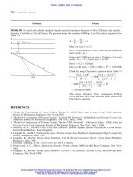
FORCE AND COUPLE RESULTANTS
AROUND THE BOUNDARY (Fig. 27-31)
The expression for force with components X and Y at
point O
The expression for couple at O
GENERALIZED PLANE STRESS
The average stress combinations assuming
z
¼ 0, a
stress free surface, i.e.
xz
¼
yz
¼ 0 at the surface
and body force potential Uðz;
"
zzÞ is independent of z
ð3 À 4vÞðzÞÀz
"
0
ð
"
zzÞÀ
"
!!ð
"
zzÞ¼2GD À
1 À 2v
2ð1 À vÞ
w
ð27-161Þ
ð3 À 4vÞðzÞÀz
"
0
ð
"
zzÞÀ
"
!!ð
"
zzÞ¼2Gðg
1
þ ig
2
Þ on C
ð27-162Þ
where g
1
and g
2
are functions of z only
X þ iY ¼Ài
h
ðzÞþz
"
0
ð
"
zzÞþ
"
!!ð
"
zzÞ
i
B
1
A
1
ð27-163Þ
N ¼ Rl
h
ÉðzÞÀz!ðzÞÀz
"
zz
0
ðzÞ
i
B
1
A
1
þ
ð
B
1
A
1
U
@z
@s
ds
ð27-164Þ
Â
o
¼
x
þ
y
ð27-165aÞ
È
o
¼
x
À
y
þ 2i
xy
ð27-165bÞ
where
Â
o
¼
1
2h
ð
h
Àh
 dz;È
o
¼
1
2h
ð
h
Àh
È dz
pav
¼
1
2h
ð
h
Àh
p
dz
Particular Formula
y
Y
N
O
X
x
ds
A
1
B
1
nb
τ
yn
τ
xn
τ
n
σ
α
FIGURE 27-31
y
y
x
x
z
2h
O
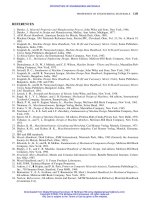
FIGURE 27-32
27.42 CHAPTER TWENTY-SEVEN
Downloaded from Digital Engineering Library @ McGraw-Hill (www.digitalengineeringlibrary.com)
Copyright © 2004 The McGraw-Hill Companies. All rights reserved.
Any use is subject to the Terms of Use as given at the website.
APPLIED ELASTICITY
The average complex displacement
The body force Eq.
@È
@z
þ
@Â
@
"
zz
þ
@É
@
"
z
¼ 0 becomes
Taking into consideration the body force, Eq. (27-167)
and other expression for F and È
o
become
The equations for generalized plane stress
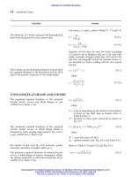
CONDITIONS ALONG A STRESS-FREE
BOUNDARY, Fig. 27-33
Adding Eqs. (27-169) and (27-170) and putting F ¼ 0
along free boundary, i.e. segment AB, the displace-
ment along AB
SOLUTION INVOLVING CIRCULAR
BOUNDARIES (Figs. 27-33 and 27-34)
From stress strain transformation rules
D
o
¼ u
o
þ iv
o
¼
1
2h
ð
h
Àh
Ddz ð27-166Þ
1
2h
ð
h
Àh
@È
@z
þ
@Â
@
"
zz
þ
@É
@z
dz ¼ 0 ð27-167aÞ
¼
@È
o
@z
þ
@Â
o
@
"
z
¼ 0
@
@
"
zz
hÂ
o
þ 2Uiþ
@È
o
@z
¼ 0 ð27-167bÞ
À
v
1 À v
@D
@z
þ
@
"
DD
@
"
zz
¼
@!
@
"
z
ð27-168aÞ
È ¼ 4G
@D
@
"
zz
ð27-168bÞ
È
o
¼ 4G
@D
o
@
"
zz
ð27-168cÞ
1 À v
1 þ v
Â
o
¼ 2G
@D
o
@z
þ
@
"
DD
@
"
zz
ð27-168dÞ
F ¼ 2fðzÞþz
"
0
ð
"
zzÞþ
"
!!ð
"
zzÞg þ
1 À 2K
1 À K
w ð27-169Þ
2GD ¼
3 À v
1 þ v
ðzÞÀz
"
0
ð
"
zzÞÀ
"
!!ð
"
zzÞÀ
1 À 2K
2ð1 À KÞ
w
ð27-170Þ
 ¼ 2
0
ðzÞþ
"
0
ð
"
zzÞÀ
1
1 À K
@w
@z
ð27-171Þ
È ¼À2fz
"
00
ð
"
zzÞþ
"
!!
0
ð
"
zzÞg À
1 À 2K
1 À K
@w
@
"
zz
ð27-172Þ
D ¼
4
E
ðzÞð27-173Þ
Â
0
¼ Â ¼
r
þ
Particular Formula
APPLIED ELASTICITY
27.43
Downloaded from Digital Engineering Library @ McGraw-Hill (www.digitalengineeringlibrary.com)
Copyright © 2004 The McGraw-Hill Companies. All rights reserved.
Any use is subject to the Terms of Use as given at the website.
APPLIED ELASTICITY
The boundary conditions are
APPLICATION OF CONFORMAL
TRANSFORMATION (Fig. 27-35)
The stress combinations after transformation
Eqs. (27-178) are related stress combinations in
rectangular coordinates x and y as
È
0
¼ F e
À2i
¼
r
À
þ 2i ¼
"
zz
z
È
where
r
¼ , z ¼ r e
i
, "zz ¼ r e
Ài
Â
0
¼ 2f
0
ðzÞþ
"
0
ð
"
zzÞg À
1
1 À K
@w
@z
ð27-174Þ
È
0
¼À2
"
zz
00
ð
"
zzÞþ
"
zz
z
"
!!
0
ð
"
zzÞ
À
1 À 2K
1 À K
"
zz
z
@w
@z
ð27-175Þ
2GD
0
¼ e
Ài
3 À v
1 þ v
ðzÞÀz
"
0
ð
"
zzÞÀ
"
!!ð
"
zzÞ
À
1 À 2K
1 À K
w ð27-176Þ
F ¼ 2
ð
s
0
ð
r
þ i
r
þ UÞ
@z
@s
ds þ constant
ð27-177aÞ
ðzÞþz
"
0
ð
"
zzÞþ
"
!!ð
"
zzÞ¼f
1
þ if
2
on C ð27-177bÞ
Â
0
¼
þ
ð27-178aÞ
È
0
¼
À
þ 2i
ð27-178bÞ
Â
0
¼ Â ð27-179aÞ
È
0
¼ È e
À2i
ð27-179bÞ
Particular Formula
C
x
A
y
B
FIGURE 27-33
y
r
x
r = constant
= constant
θ
θ
FIGURE 27-34
27.44 CHAPTER TWENTY-SEVEN
Downloaded from Digital Engineering Library @ McGraw-Hill (www.digitalengineeringlibrary.com)
Copyright © 2004 The McGraw-Hill Companies. All rights reserved.
Any use is subject to the Terms of Use as given at the website.
APPLIED ELASTICITY
An explanation for e
À2i
Using Eqs. (27-179a) and (27-179b), and Eqs. (27-171)
and (27-172), when these are no body forces, letting
ðzÞ¼
1
ðÞ and !ðzÞ¼!
1
ðÞ
The transformation of a given boundary in the z-
plane into the unit circle in the -plane
Using polar coordinates (, #), the stress components
become
Using polar coordinates Eqs. (27-180a) and (27-181)
in terms of complex potentials become
where
z ¼ zðÞ¼f ð; Þþigð; Þ
¼ þi
f ð; Þ and gð; Þ are real and imaginary parts of zðÞ
e
À2i
¼
"
zz
0
ð
"
Þ=z
0
ðÞð27-179cÞ
or
Â
0
¼ 2
0
1
ðÞ
d
dz
þ
"
0
1
; ð
"
Þ
d
"
d
"
zz
ð27-180aÞ
Â
0
¼ 2
0
1
ðÞ
z
0
ðÞ
þ
"
0
1
; ð
"
Þ
"
zz
0
ð
"
Þ
ð27-180bÞ
È
0
¼À
2
z
0
ðÞ
n
zðÞh
"
00
"
0
1
ð
"
Þþ
"
0
"
00
1
ð
"
Þi þ
"
!!
0
1
ð
"
Þ
o
ð27-181aÞ
or
È
0
¼À
2
z
0
ðÞ
1
zðÞ
"
0
1
; ð
"
Þ
"zz
0
ð
"
Þ
þ
"
!!
0
1
; ðÞ
()
ð27-181bÞ
Â
00
¼
þ
#
ð27-182aÞ
È
00
¼
þ
#
À 2i
#
ð27-182bÞ
where Â
00
¼ Â
0
and È
00
¼ È
0
e
À2i#
¼
"
È
0
:
Â
00
¼ 2
0
ðÞ
z
0
ðÞ
þ
"
0
ð
"
Þ
"
zz
0
ð
"
Þ
"#
ð27-183Þ
È
00
¼À
2
"
z
0
ðÞ
h
zðÞh
"
00
"
0
1
ð
"
Þþ
"
0
"
00
1
ð
"
Þi þ
"
!!
0
ð
"
Þ
i
ð27-184aÞ
È
00
¼
2
"
z
0
ðÞ
zðÞ
"
0
ð
"
Þ
"
zz
0
ð
"
Þ
þ
"
!!
0
ð
"
Þ
"#
ð27-184bÞ
Particular Formula
ϑ
ϑ
y
r
O
P
x
(a) z - plane
= constant
η
= constant
ξ
α
O
Q
(b)
ϕ - plane
= constant
= constant
ρ
η
ρ
ξ
O
(c)
= constant
ξ
τ
ξ
η
σ
ξ
η
ξ
FIGURE 27-35
APPLIED ELASTICITY
27.45
Downloaded from Digital Engineering Library @ McGraw-Hill (www.digitalengineeringlibrary.com)
Copyright © 2004 The McGraw-Hill Companies. All rights reserved.
Any use is subject to the Terms of Use as given at the website.
APPLIED ELASTICITY
Rectangular plate under all round tension
Value of complex potentials ðzÞ and !ðzÞ assumed
From stress combination Eqs. (27-156c) and (27-157)
The stress
x
and
y
after equating real and imaginary
parts
The displacement from Eq. (27-158) after equating
real and imaginary parts
Rectangular plate under plane flexure
Assume values of complex potentials ðzÞ and !ðzÞ as
ðzÞ¼
1
2
Tz; !ðxÞ¼0 ð27-185Þ
 ¼ 2f
0
ðzÞþ
"
0
ð
"
zzÞg þ
1
1 À v
@w
@z
¼ 2½
1
2
T þ
1
2
T¼2T ð27-156cÞ
È ¼À2fz
"
00
ð
"
zzÞþ
"
!!
0
ð
"
zzÞg þ
1 À 2v
1 À v
@w
@
"
zz
ð27-157Þ
where  ¼
x
þ
y
and È ¼
x
À
y
þ 2i
xy
x
¼ T;
y
¼ T;
xy
¼ 0 ð27-186Þ
2GD ¼ð3 À 4vÞðzÞÀz
"
0
ð
"
zzÞÀ
"
!!ð
"
zzÞ
þ
1 À 2v
2ð1 À vÞ
w ð27-158Þ
D ¼
T
E
ð1 À vÞðx þ iyÞ¼u þ i
u ¼
T
E
ð1 À vÞx; ¼
T
E
ð1 À vÞy ð27-187Þ
ðzÞ¼Az
2
!ðzÞ¼Bz
2
Choose A and B, which may be complex, so that edges
y ¼Æb are stress free.
Particular Formula
y
T
x
z
y
y
dy
T
a a
2b
2h
T
T
FIGURE 27-36
2b
M
b
M
b
a a
y
y
σ
x
x
σ
xy
τ
xy
τ
FIGURE 27-37
27.46 CHAPTER TWENTY-SEVEN
Downloaded from Digital Engineering Library @ McGraw-Hill (www.digitalengineeringlibrary.com)
Copyright © 2004 The McGraw-Hill Companies. All rights reserved.
Any use is subject to the Terms of Use as given at the website.
APPLIED ELASTICITY
Boundary conditions
From stress combinations Eqs. (27-156) and (27-157)
boundary conditions
The bending moment
The values of complex potentials ðzÞ¼Az
2
and
!ðzÞ¼Bz
2
are
The displacement from Eq. (27-158)
Thick cylinder under internal and external
pressure
Values of complex potentials ðzÞ and !ðzÞ assumed
using boundary conditions at r ¼ a or d
i
=2 and
r ¼ b or d
o
=2 with no body forces, assuming internal
pressure p
i
, external pressure p
o
, values of A and B
in Eq. (27-189), which are real, can be found. From
Eqs. (27-174) and (27-175)
The expressions for
and
r
at any radius
Rotating solid disk and hollow disk of
uniform thickness rotating at ! rad/s
Values of complex potentials ðzÞ and !ðzÞ assumed
0
ðzÞþ
"
0
ð
"
zzÞþ
"
zz
00
ðzÞþ!
0
ðzÞ¼
y
þ i
xy
ð27-156Þ
y
¼ 0,
xy
¼ 0 throughout the plate
A ¼ iC and B ¼ÀiC where C is real
 ¼
0
x
þ
0
y
¼
0
x
¼À8Cy
M
b
¼
ð
b
Àb
x
2hy dy ¼À8CI ð27-188Þ
where
I ¼ moment of inertia about oz
C ¼À
M
b
8I
ðzÞ¼À
iM
b
8I
z
2
; !ðzÞ¼
iM
b
8I
z
2
ð27-188aÞ
D ¼
1
2G
h
ð3 À 4vÞðzÞÀz
"
0
ð
"
zzÞÀ
"
!!ð
"
zzÞ
i
¼ u þiv
when body forces are zero
Substituting the values of ðzÞ and !ðzÞ in the above,
u and v can be determined.
ðzÞ¼Az and !ðzÞ¼
B
z
ð27-189aÞ
where A and B are real
1
2
½Â
0
þ È
0
¼
r
þ i
r
¼
0
ðzÞþ
"
0
ð"zzÞ
À z
"
00
ðzÞÀ
z
"
zz
"
!!
0
ð
"
zzÞð27-189bÞ
The equations for
and
r
are given in Eqs. (27-101b)
and (27-101a) respectively.
ðzÞ¼Cz and !ðzÞ¼
B
z
ð27-189cÞ
where C and B are real
Particular Formula
APPLIED ELASTICITY
27.47
Downloaded from Digital Engineering Library @ McGraw-Hill (www.digitalengineeringlibrary.com)
Copyright © 2004 The McGraw-Hill Companies. All rights reserved.
Any use is subject to the Terms of Use as given at the website.
APPLIED ELASTICITY
Using boundary conditions at ð
r
Þ
r ¼b
¼ 0 and
ð
r
Þ
r ¼0
6¼ 0 for solid disk ð
r
Þ
r ¼a
¼ 0 and
ð
r
Þ
r ¼b
¼ 0 for hollow disc taking into consideration
body forces, values of C and B in Eq. (27-189c) which
are real can be found
The radial displacements at the boundaries
Large plate under uniform uniaxial tension
with a centrally located unstressed circular
hole
Values of complex potentials ðzÞ and !ðzÞ assumed
Using Eq. (27-189b) and above complex potentials
Using boundary condition at r ¼ a
The new values of ðzÞ and !ðzÞ
Using Eqs. (27-174), (27-175) and after equating the
real and imaginary parts, the stress components are
x
TT
y
aA
A
θ
FIGURE 27-38
Refer Eqs. (27-126), (27-127) and (27-128) to (27-131)
ðu
r
Þ
r ¼a
¼
!
2
a
4E
fð1 À vÞa
2
þð3 þ vÞb
2
gð27-189dÞ
ðu
r
Þ
r ¼b
¼
!
2
b
4E
fð1 À vÞb
2
þð3 þ vÞa
2
gð27-189eÞ
ðzÞ¼
Tz
4
þ
A
z
ð27-190Þ
!ðzÞ¼À
1
2
Tz þ
B
z
þ
C
z
3
where A, B and C are real
r
À i
r
¼
1
2
T À
3A
z
2
þ
1
2
T
z
"
zz
þ
B
z
"
zz
þ
3C
z
3
"
zz
ð27-190aÞ
ð
r
À i
r
Þ
r ¼a
¼
1
2
T þ
B
a
2
þ
1
2
T þ
A
a
2
e
2i
þ
3C
a
4
À
3A
a
2
e
2i
ð27-190bÞ
A ¼
1
2
Ta
2
; B ¼À
1
2
Ta
2
; C ¼
1
2
a
4
ð27-190cÞ
since hole is stress free
ðzÞ¼
Tz
4
þ
1
2
Ta
2
z
ð27-190dÞ
!ðzÞ¼À
1
2
Tz À
Ta
2
4
þ
a
4
2z
3
ð27-190eÞ
r
¼
1
2
T
1 À
a
2
r
2
þ
1 À
4a
2
r
2
þ
3a
4
r
4
cos 2
"#
ð27-191Þ
¼
1
2
T
1 þ
a
2
r
2
À
1 þ
3a
4
r
4
cos 2
"#
ð27-192Þ
r
¼À
1
2
T
1 þ
2a
2
r
2
À
3a
4
r
4
sin 2 ð27-193Þ
Particular Formula
27.48 CHAPTER TWENTY-SEVEN
Downloaded from Digital Engineering Library @ McGraw-Hill (www.digitalengineeringlibrary.com)
Copyright © 2004 The McGraw-Hill Companies. All rights reserved.
Any use is subject to the Terms of Use as given at the website.
APPLIED ELASTICITY
The
,
r
and
r
at r ¼ a
The maximum tangential stress
The stress concentration factor
Large plate containing a circular hole under
uniform pressure
Values of complex potentials ðzÞ and !ðzÞ assumed
From Eqs. (27-174) and (27-175) in the absence of
body forces
Boundary conditions are
The new complex potentials
The stress components are
The displacement from Eq. (27-176)
Large plate containing a circular hole filled
by an oversize disk
1. Rigid Disk
The radius of disk r
d
ð
r
Þ
r ¼a
¼ð
r
Þ
r ¼a
¼ 0 ð27-194aÞ
ð
Þ
r ¼a
¼ Tð1 À 2 cos 2Þð27-194bÞ
max
¼ð
Þ
r ¼a
¼ 3T ð27-194cÞ
K
¼
ð
Þ
max
T
¼
3T
T
¼ 3 ð27-195Þ
ðzÞ¼0; !ðzÞ¼
A
z
ð27-196Þ
Â
0
¼ 2f
0
ðzÞþ
"
0
ð
"
zzÞg ¼
r
þ
¼ 0 ðaÞ
È
0
¼ 2
"
zz
"
00
ð
"
zzÞþ
"
zz
z
"
!!
0
ð
"
zzÞ
¼
r
À
þ 2i
r
¼
2A
r
2
ðbÞ
ð
r
Þ
r ¼a
¼Àp ¼
2A
a
2
A ¼Àpa
2
ðcÞ
ðzÞ¼0; !ðzÞ¼À
pa
2
z
ðdÞ
r
¼À
pa
2
r
2
;
r
¼ 0 ð27-197Þ
¼À
r
¼
pa
2
r
2
2GD
0
¼ 2Gðu
r
þ iu
Þ¼e
Ài
À
A
"
zz
¼À
A
r
ðu
r
޼A
2Gr
; u
¼ 0 ð27-198Þ
ðu
r
Þ
r ¼a
¼
pa
2G
r
d
¼ að1 þ"ÞðaÞ
where a ¼ radius of hole
Particular Formula
APPLIED ELASTICITY
27.49
Downloaded from Digital Engineering Library @ McGraw-Hill (www.digitalengineeringlibrary.com)
Copyright © 2004 The McGraw-Hill Companies. All rights reserved.
Any use is subject to the Terms of Use as given at the website.
APPLIED ELASTICITY
From first of Eq. (27-198), the radial displacement
The stress components
2. Elastic Disk
The complex potential for all round pressure on the
disk
The displacement from Eq. (27-176)
The radial displacement of plate
The pressure between disc and plate
Elliptical hole in a large plate under tension
(Fig. 27-39)
The expression for transformation
u
r
¼ a" ¼À
A
2Ga
or A ¼À2Ga
2
" ðbÞ
r
¼À
¼À2G"
a
2
r
2
ðcÞ
r
¼ 0 ðdÞ
1
ðzÞ¼À
1
2
pz; !
1
ðzÞ¼0 ðeÞ
2G
1
D
0
¼ 2G
1
ðu
r1
þ iu
1
Þ¼e
Ài
Àð1 À vÞpz
1 þ v
¼À
Àpð1 À v
1
Þpa
1 þ v
1
ð f Þ
u
r1
¼
Àpð1 À v
1
Þa
E
1
ðgÞ
where subscript 1 for disk and 2 for plate
u
r2
¼
pa
2G
2
ðhÞ
p ¼
E
1
E
2
E
1
ð1 þ v
2
ÞþE
2
ð1 À v
1
Þ
ð27-198Þ
z ¼ C
þ
m
; m < 1 ð27-199Þ
Transforms the outside of an ellipse of semiaxes a and
b in the z-plane into the outside of a unit circle r in the
-plane, provided
C ¼
1
2
ða þ bÞ; m ¼
a À b
a þ b
ð27-200aÞ
z
C
¼ e
i#
þ m e
Ài#
¼ð1 þmÞcos # þð1 À mÞi sin # ð27-200bÞ
z ¼
a þ b
2
2a
a þ b
cos # þ i
2b
a þ b
sin #
ð27-200cÞ
or x þ iy ¼ a cos # þib sin # ð27-200dÞ
# ¼ eccentric angle around the ellipse
Particular Formula
27.50 CHAPTER TWENTY-SEVEN
Downloaded from Digital Engineering Library @ McGraw-Hill (www.digitalengineeringlibrary.com)
Copyright © 2004 The McGraw-Hill Companies. All rights reserved.
Any use is subject to the Terms of Use as given at the website.
APPLIED ELASTICITY
The points at which the transformation ceases to be
conformal are
The boundary condition at the stress free ellipse
The boundary condition in terms of
Eq. (27-203) on unit circle becomes
The complex potentials for an infinite plate without a
hole acted upon by uniaxial tension at an angle to
the x-axis in the z-plane and -plane
The complex potentials for an infinite plate with stress
free elliptic hole subject to tension at an angle to the
x-axis in -plane
z
0
ðÞ¼0 ð27-201aÞ
z
0
ðÞ¼C
1 À
m
2
¼ 0 ð27-201bÞ
¼Æ
ffiffiffiffi
m
p
; since m < 1
ðzÞþz
"
0
ð
"
zzÞþ
"
!!ð
"
zzÞ¼f
1
þ if
2
ð27-202Þ
on the boundary of ellipse ¼ 0
1
ðÞþzðÞ
"
0
1
ð
"
Þ
"
zz
0
ð
"
Þ
þ
"
!!
1
ð
"
Þ¼0
or
"
zz
0
ðÞ
1
ðÞþzðÞ
"
0
1
ð
"
Þþ
"
zz
0
ð
"
Þþ
"
zz
0
ð
"
Þ
"
!!
1
ð
"
Þ¼0
ð27-203Þ
"
zz
0
ð"Þ
1
ðÞþzðÞ
"
0
1
ð"Þþ
"
zz
0
ð"Þ
"
!!
0
1
ð"Þ¼0
or
"
zz
0
1
1
ðÞþzðÞ
"
0
1
1
þ
"
zz
0
1
"
!!
1
1
¼ 0
ð27-204Þ
where ¼ ;
"
¼ " ¼
1
on since " ¼ 1 on unit
circle
ðzÞ¼
1
4
Tz;!ðzÞ¼À
1
2
Tz e
À2i
on z plane
ð27-205aÞ
z ¼ Cð þm=Þ!C and z
0
ðÞ¼C
1 À
m
2
! C at in -plane
1
ðÞ¼
1
4
TC; !
1
ðÞ¼À
1
2
TC e
À2i
ð27-205bÞ
1
ðÞ¼
1
4
TC
þ
A
þ
B
2
þ
C
3
þÁÁÁ
ð27-206aÞ
z
0
ðÞ!
1
ðÞ¼À
1
2
TC
2
e
À2i
þ
D
1
þ
E
1
2
þ
F
1
3
þÁÁÁ
ð27-206bÞ
Particular Formula
z = x + iy
(a) z - Plane (b) ζ - Plane
y
x
1
a
a
α
η
ϑ
ξ
ζ = ξ+iη = e
i
ϑ
b
b
T
T
s
η
FIGURE 27-39
APPLIED ELASTICITY
27.51
Downloaded from Digital Engineering Library @ McGraw-Hill (www.digitalengineeringlibrary.com)
Copyright © 2004 The McGraw-Hill Companies. All rights reserved.
Any use is subject to the Terms of Use as given at the website.
APPLIED ELASTICITY
Using Eqs. (27-206) in Eqs. (27-204), after equating
coefficients of powers of or (since
E
1
¼ B ¼ C ¼ 0, D
1
¼ 1 þm
2
À 2Me
2i
, F
1
¼Àe
2i
,
A ¼ 2e
2i
À mÞ
The tangential stress on the boundary of elliptical
hole from Eq. (27-183) Â
00
¼
#
þ
where
¼ 0
after equating to real part of right hand side of
equation and simplification (Fig. 27-39)
The tangential stress on the boundary of elliptical
hole for ¼ 0 (Fig. 27-40)
The maximum tangential stress
# max
on the contour
of any elliptical hole for any value of m ¼
a À b
a þ b
and
c ¼
1
2
ða þ bÞ will be at # ¼Æ
2
If a ¼ b in Eq. (27-209), then the ellipse becomes a
circle
The stress concentration factor
By taking ¼ 458 with T ¼ÀS, and ¼À458 with
T ¼þS, and on adding these solutions, a solution
for pure shear S applied to an infinite flat plate with
an elliptical hole at infinity is obtained. The shear
will be parallel to the axes of the ellipse with
around the elliptical hole is given by
MUSKHELISHVILI’S DIRECT METHOD
In this method that a hole L can be transformed
conformally into a unit circle in the -plane so
that outside of the hole is mopped on the inside of
(Fig. 27-41)
The form of the conformal transformation will be
If the loading of the plate at infinity is given by the
complex potential
Ã
ðÞ, !ðÞ
Ã
, the full complex
potentials which will also satisfy the condition
around the hole, can be written as
1
ðÞ¼
1
4
TC þ
2e
2i
À m
*+
ð27-206cÞ
!
1
ðÞ¼À
1
2
TC
*
e
À2i
þ
1 þ m
2
À 2m e
2i
À
e
2i
3
1 À
m
2
+
ð27-206dÞ
#
¼ T
1 À m
2
þ 2m cos 2 À 2 cos 2ð# À Þ
1 þ m
2
À 2m cos 2#
ð27-207Þ
#
¼ T
1 À m
2
þ 2m À 2 cos 2#
1 þ m
2
À 2n cos 2#
ð27-208Þ
ð
#
Þ
max
¼ T
3 À m
1 þ m
¼ T
1 þ
2b
a
ð27-209Þ
ð
v
Þ
max
¼ 3T ð27-209aÞ
K
¼
ð
v
Þ
max
T
¼ 3 ð27-209bÞ
¼ S
4 sin 2
1 À 2m cos 2 þ m
2
ð27-210Þ
z ¼ C
1
þ e
1
þe
2
2
þ e
3
3
þÁÁÁþe
n
n
ð27-211Þ
ðÞ¼
Ã
ðÞþ
o
ðÞð27-212Þ
!ðÞ¼!
Ã
ðÞþ!
o
ðÞð27-213Þ
where
o
ðÞ¼
X
1
o
a
n
n
;!
o
ðÞ¼
X
1
o
b
n
n
ð27-213aÞ
Particular Formula
27.52 CHAPTER TWENTY-SEVEN
Downloaded from Digital Engineering Library @ McGraw-Hill (www.digitalengineeringlibrary.com)
Copyright © 2004 The McGraw-Hill Companies. All rights reserved.
Any use is subject to the Terms of Use as given at the website.
APPLIED ELASTICITY
The boundary condition around a stress free hole
assuming no body forces is given by (refer to Eqs.
(27-203) and (27-204))
Substituting the complex potentials given by Eqs.
(27-212), in Eq. (27-214)
Using Harnack’s theorem, residue theorem and
Cauchy’s integral, multiplying by
1
2i
d
À
and
integrating around Eq. (27-214) can be written as
The complex potential
o
ðÞ from Eq. (27-216) is
ðÞþ
zðÞ
"
zz
0
1
"
0
1
þ
"
!!
1
¼ 0 ð27-214Þ
o
ðÞþ
zðÞ
"
zz
0
1
"
0
o
1
þ
"
!!
o
1
¼ f
1
þ if
2
ð27-215aÞ
where
f
1
þ if
2
¼À
Ã
ðÞþ
zðÞ
"
zz
0
1
"
0Ã
1
þ
"
!!
Ã
1
2
6
4
3
7
5
ð27-215bÞ
1
2i
ð
o
ðÞ
À
d þ
1
2i
ð
zðÞ
"
zz
0
1
"
0
o
1
À
d
þ
1
2i
ð
"
!!
o
1
À
d ¼
1
2i
ð
f
1
þ if
2
À
d
ð27-216Þ
o
ðÞþ
1
2i
ð
zðÞ
"
0
o
1
"
zz
0
1
ð À Þ
d ¼
1
2i
ð
f
1
þ if
2
À
d
ð27-217Þ
Particular Formula
S
S
S
S
S
S
θ
S
a
b
45
45
FIGURE 27-40
y
x
L
z-Plane
o
η
ξ
ζ-Plane
o
ζ
η
FIGURE 27-41
APPLIED ELASTICITY
27.53
Downloaded from Digital Engineering Library @ McGraw-Hill (www.digitalengineeringlibrary.com)
Copyright © 2004 The McGraw-Hill Companies. All rights reserved.
Any use is subject to the Terms of Use as given at the website.
APPLIED ELASTICITY
Taking conjugate of Eq. (27-215), remembering that
" ¼ 1 and multiplying by
1
2i
d
À
and integrating
around
The complex potential !
o
ðÞ can be found after
substituting the value of
o
ðÞ Eq. (27-218) which
can be evaluated from Eq. (27-217)
Stress free square hole in a flat plate under
uniform uniaxial tension (Fig. 27-42)
The form of the conformal transformation will be
The known complex potential in this case
After substituting
Ã
ðÞ and !
Ã
ðÞ from Eqs. (27-221)
and (27-222) into Eq. (27-215)
After substituting the value of f
1
þ if
2
from
Eq. (27-223) in Eq. (21-217) and simplification
Substituting the value of
o
ðÞ from Eq. (27-224) in
Eq. (27-219) and after simplification
1
2i
ð
"
o
1
À
d þ
1
2i
ð
"
zz
1
z
0
ðÞ
0
o
ðÞ
À
d
þ
1
2i
ð
!
o
ðÞ
À
d ¼
1
2i
ð
f
1
À if
2
À
d
ð27-218Þ
1
2i
ð
"zz
1
z
0
ðÞ
0
o
ðÞ
À
d þ !
o
ðÞ¼
1
2i
ð
f
1
À if
2
À
d
ð27-219Þ
y
T
T
x
d
FIGURE 27-42
z ¼ C
1
À
3
6
ð27-220Þ
Ã
ðÞ¼
1
4
TC
1
À
3
6
ð27-221Þ
!
Ã
ðÞ¼À
1
2
TC
1
À
3
6
ð27-222Þ
f
1
þ if
2
¼À
1
4
TC
2
À 2 À
3
3
þ
1
3
3
ð27-223Þ
o
ðÞ¼TC
3
7
þ
1
12
3
ð27-224Þ
!
o
ðÞ¼À
1
4
TC
2 þ
1
3
3
À
1
3
1 À 6
4
2 þ
4
 TC
3
7
þ
2
4
"#
þ
1
14
TC
ð27-225Þ
Particular Formula
27.54 CHAPTER TWENTY-SEVEN
Downloaded from Digital Engineering Library @ McGraw-Hill (www.digitalengineeringlibrary.com)
Copyright © 2004 The McGraw-Hill Companies. All rights reserved.
Any use is subject to the Terms of Use as given at the website.
APPLIED ELASTICITY
The full complete complex potentials after simplifi-
cation
The tangential stress around the square hole
By adding more terms to the expression for trans-
formation
The radius r will be rounded of
For graph of
#
=T versus # in degrees
Stress free square hole in a flat plate under
pure bending (Fig. 27-44)
The conformal transformation for plate with a square
hole such that the diagonals along the coordinate axes
as shown in Fig. 27-44
The known complex potentials from Eqs. (27-188a)
ðÞ¼TC
3
7
þ
1
4
1
þ
1
24
3
ð27-226Þ
!ðÞ¼ÀTC
1
2
þ
91 À78
3
84ð2 þ
4
Þ
ð27-227Þ
#
¼ Rl: 4
0
ðÞ
z
0
ðÞ
ð27-228Þ
z ¼ C
1
À
1
6
3
þ
1
56
7
ð27-228aÞ
the radius becomes r ¼ 0:025d
z ¼ C
1
À
1
6
3
þ
1
56
7
À
1
176
11
ð27-228bÞ
the radius becomes r ¼ 0:014d
Refer to Fig. 27-43.
z ¼ C
1
þ
1
6
3
ð27-229Þ
Ã
ðzÞ¼À
iM
b
8I
z
2
; !
Ã
ðzÞ¼
iM
b
8I
z
2
ð27-188aÞ
Particular Formula
8
20 40
60
ϑ
T
d
r
T
Square Hole
r = 0.06 d
r = 0.025 d
r = 0.014 d
80
- Degrees
90
I
I
I
II
II
II
III
III
III
6
4
2
0
2
4
ϑ
FIGURE 27-43
M
b
M
b
FIGURE 27-44 Flat plate with stress-free square
hole under pure bending.
APPLIED ELASTICITY
27.55
Downloaded from Digital Engineering Library @ McGraw-Hill (www.digitalengineeringlibrary.com)
Copyright © 2004 The McGraw-Hill Companies. All rights reserved.
Any use is subject to the Terms of Use as given at the website.
APPLIED ELASTICITY
The complete complex potentials in -plane will be of
the form
From Eq. (27-217)
From Eq. (27-219)
The full complex potentials become often simplifying
After knowing full complex potentials, the tangential
stress at various angles around the hole/cutout can be
calculated
For graphs of
v
=ðM
b
c=IÞ versus # degree
Large plate containing an elliptical hole
subjected to uniform pressure (Fig. 27-46)
The expression for transformation
The complex potential at infinity
The required complex potentials
Boundary conditions
ðÞ¼À
iM
b
C
2
8I
1
þ
1
6
3
2
þ
o
ðÞð27-230aÞ
!ðÞ¼
iM
b
C
2
8I
1
þ
1
6
3
2
þ !
o
ðÞð27-230bÞ
o
ðÞ¼
iM
b
C
2
8I
4
3
2
À
1
3
4
þ
1
36
6
ð27-231Þ
!
o
ðÞÀ
1
2
1 þ 6
4
2 À
4
0
o
ðÞ
¼À
iM
b
C
2
8I
4
3
2
À
1
3
4
þ
1
16
6
À
37
18
ð27-232Þ
ðÞ¼À
iM
b
C
2
8I
1
2
À
2
þ
1
3
4
ð27-233Þ
!ðÞ¼
iM
b
C
2
8I
18 þ 45
2
À 31
4
þ 36
6
À 15
8
9
2
ð2 À
4
Þ
ð27-234Þ
Refer to Fig. 27-45.
z ¼ C
þ
m
; m < 1 ð27-199Þ
where
C ¼
1
2
ða þ bÞ; m ¼
a À b
a þ b
Refer to other details under Eq. (27-199)
Ã
ðÞ¼!
Ã
ðÞ¼0 ð27-235aÞ
ðÞ¼
X
1
0
a
n
n
; !ðÞ¼
X
1
0
b
b
n
ð27-235bÞ
n
¼
¼Àp;
ns
¼ 0 around the hole ð27-236Þ
Particular Formula
27.56 CHAPTER TWENTY-SEVEN
Downloaded from Digital Engineering Library @ McGraw-Hill (www.digitalengineeringlibrary.com)
Copyright © 2004 The McGraw-Hill Companies. All rights reserved.
Any use is subject to the Terms of Use as given at the website.
APPLIED ELASTICITY
From Eq. (27-117b)
Expressing Eq. (27-237) in -plane at all points of
Multiplying Eq. (27-238) by
1
2i
@
À
[Considering the first of these integrals, one has to
remember that is now a boundary to the region
external to the unit circle. Thus it is necessary to con-
sider an integration around a contour consisting of
together with C circle
0
of large radius R joined by
two close paths AB and CD, Fig. 27-46]
Using Cauchy’s integral, Harnack’s theorem and
residue theorem, Eq. (27-239) gives the expression
for ðÞ
ðzÞþ2
"
0
ð
"
zzÞþ
"
!!ð
"
zzÞ
¼ð
n
þ
ns
Þ
@z
@s
ds
¼Àpz at all points on the ellipse ð27-237Þ
ðÞþ
zðÞ
"
zz
0
1
"
0
1
þ
"
!!
1
¼ÀpzðÞ
ðÞþ
2
þ mðÞ
ð1 À m
2
Þ
"
0
1
þ
"
!!
1
¼ÀpC
þ
m
ð27-238Þ
1
2i
ð
ðÞ@
À
þ
1
2i
ð
2
þ m
ð1 À m
2
Þ
"
0
1
À
d
þ
1
2i
ð
"
!!
1
d
À
¼
ÀpC
2i
ð
þ
m
À
d
ð27-239Þ
ðÞ¼À
pCm
ð27-240Þ
Particular Formula
2
1
0
20
40
60
80 90
1
2
3
4
5
6
III
III
I
I
II
II
M
b
ϑ
M
b
I - Second moment of inertia
= Angle form z-axis to a point
on hole boundary
x
III
II
I
FIGURE 27-45
b
p
p
p
a
n
B
(a)
(b)
C
D
R
A
γ
γ
FIGURE 27-46
APPLIED ELASTICITY
27.57
Downloaded from Digital Engineering Library @ McGraw-Hill (www.digitalengineeringlibrary.com)
Copyright © 2004 The McGraw-Hill Companies. All rights reserved.
Any use is subject to the Terms of Use as given at the website.
APPLIED ELASTICITY
Taking conjugate of Eq. (27-239) and integrating
around , the expression for !ðÞ
The stress can be obtained by making use of
Eq. (27-183) for Â
00
and (27-184b) for È
00
and equating
real parts on both sides of equation
The tangential stress around by elliptical hole from
Eq. (27-243)
Large flat plate under uniform uniaxial
tension with a circular hole whose edge is
rigidly fixed (Fig. 27-49)
The edge of the hole r ¼ a is held fixed by a rigid
circular ring to which the material of the plate adheres
at all points
The boundary condition is given by T
The complex potential form of displacement for
generalized plane stress problem from Eqs. (27-170)
when there are no body forces
!ðÞ¼À
pC
À
pCm
1 þ m
2
2
À m
ð27-241Þ
½
¼1
¼Àp from boundary condition ð27-242Þ
½Â
00
¼1
¼ 4Rl
0
ðÞ
z
0
ðÞ
¼1
¼
#
þ
¼
4pmðcos 2# À mÞ
1 þ m
2
À 2m cos 2#
ð27-243Þ
#
¼
4#mðcos 2v À mÞ
1 þ m
2
À 2m cos 2#
þ p ð27-244Þ
or
#
¼ p
1 þ 2m cos 2# À 3m
2
1 À 2m cos # þ m
2
ð27-245Þ
½D
r ¼a
¼ 0 for all # ð27-246aÞ
2GD ¼
3 À v
1 þ v
ðzÞÀz
"
0
ð
"
zzÞÀ
"
!!ð
"
zzÞ¼0 ð27-246bÞ
or
KðzÞÀz
"
0
ð
"
zzÞÀ
"
!!ð
"
zzÞ¼0onr ¼ a ð27-246cÞ
where
K ¼
3 À v
1 þ v
KðÞÀzð
"
Þ
0
ðÞ
z
0
ð
"
Þ
À
"
!!ð
"
Þ¼0 in terms of
ð27-246dÞ
Particular Formula
T
T
x
y
a
θ
FIGURE 27-47
27.58 CHAPTER TWENTY-SEVEN
Downloaded from Digital Engineering Library @ McGraw-Hill (www.digitalengineeringlibrary.com)
Copyright © 2004 The McGraw-Hill Companies. All rights reserved.
Any use is subject to the Terms of Use as given at the website.
APPLIED ELASTICITY
The conformal transformation for this problem can
be taken as
The full complex potentials in this case can be taken
as
The condition to be satisfied on " ¼ 1by
o
ðÞ and
!
o
ðÞ is
Multiplying Eq. (27-249) by
1
2i
d
À
and integrating
around , after simplification
Multiplying the conjugate of Eq. (27-229) by
1
2i
d
À
and integrating around and after simplifi-
cation, expression for !
o
ðÞ
The full complex potentials are
From the Eqs. (27-182a) and (27-182b) for Â
00
and È
00
,
the following stress components are
TORSION (Fig. 25-49)
The angle of twist , which is proportional to the
distance of cross-section from the fixed end
z ¼
a
ð27-247Þ
ðÞ¼
1
4
Ta
þ
o
ðÞð27-248aÞ
!ðÞ¼À
1
2
Ta
þ !
o
ðÞð27-248bÞ
where first terms in each of the above equations is
for stress state at infinity
K
o
ðÞÀ
zðÞ
z
0
1
"
0
o
1
À "!!
o
1
¼À
1
4
TðK À 1Þ
a
À
1
2
Ta ð27-249Þ
o
ðÞ¼À
Ta
2K
ð27-250Þ
!
o
ðÞ¼
1
4
Ta
ðK À 1Þ À
2
K
3
ð27-251Þ
ðÞ¼
1
4
Ta
1
À
2
K
ð27-252aÞ
!ðÞ¼À
1
2
T
a
þ
1
4
Ta
ðK À 1Þ À
2
K
3
ð27-252bÞ
¼
1
4
TðK þ 1Þ
1 þ
2
K
cos 2#
ð27-253Þ
#
¼
1
4
Tð3 À KÞ
1 þ
2
K
cos 2#
ð27-254Þ
#
¼
1
2
T
K þ 1
K
sin 2# ð27-255Þ
¼ z ð27-256Þ
where ¼ angle of twist per unit length
Particular Formula
APPLIED ELASTICITY
27.59
Downloaded from Digital Engineering Library @ McGraw-Hill (www.digitalengineeringlibrary.com)
Copyright © 2004 The McGraw-Hill Companies. All rights reserved.
Any use is subject to the Terms of Use as given at the website.
APPLIED ELASTICITY
Pðx; y; zÞ is a point in a section of bar z-distance from
fixed end (Fig. 27-48) and it is displaced to a new point
P
0
ðx þ u; y þ v; z þ wÞ after deformation due to twist
such that OP % OP
0
% r
The displacement of point P in x-direction assuming
that is small such that cos ¼ 1 and sin %
The displacement of point P in y-direction
The warping of bar, which is invariant with z and is
defined by a function
The component of strains from Eqs. (27-40) and
(27-41)
The stress components from Eqs. (27-34) and (27-37)
The equations of equilibrium from Eqs. (27-11)
u ¼ r cosð þ ÞÀr cos %Ày ¼Àzy ð27-257Þ
v ¼ r sinð þ ÞÀr sin % x ¼ zx ð27-258Þ
w ¼ ðx; yÞð27-259Þ
where ðx; yÞ is a function of x and y only
"
x
¼ "
y
¼ "
z
¼
xy
¼ 0 ð27-260aÞ
yz
¼
@w
@x
þ
@u
@z
¼ G
@
@x
À y
ð27-260bÞ
xz
¼
@w
@y
þ
@v
@z
¼ G
@
@y
þ x
ð27-260cÞ
x
¼
y
¼
z
¼
xy
¼ 0 ð27-261aÞ
xz
¼ G
@
@x
À y
ð27-261bÞ
yz
¼ G
@
@y
þ x
ð27-261cÞ
@
x
@x
þ
@
xy
@y
þ
@
xz
@z
þ F
bx
¼ 0 ð27-11aÞ
@
y
@y
þ
@
yz
@z
þ
@
yx
@x
þ F
by
¼ 0 ð27-11bÞ
@
z
@z
þ
@
zx
@x
þ
@
zy
@y
þ F
bz
¼ 0 ð27-11cÞ
Particular Formula
y
x
α
z
M
t
M
t
O
Fixed
End
FIGURE 27-48 Torsion of prismatic bar.
O
y
x
r
u
v
P(x, y)
P’(x+u, y+ν)
α
β
FIGURE 27-49 Shows a cross-section of twisted bar in xy-
plane.
27.60 CHAPTER TWENTY-SEVEN
Downloaded from Digital Engineering Library @ McGraw-Hill (www.digitalengineeringlibrary.com)
Copyright © 2004 The McGraw-Hill Companies. All rights reserved.
Any use is subject to the Terms of Use as given at the website.
APPLIED ELASTICITY
Neglecting body forces in z-direction, Eq. (27-11)
yields after substituting the Eqs. (27-261b) and
(27-261c) in it
From the equilibrium condition of the surface
Eq. (27-7)
When surface forces are absent F
Nx
¼ F
Ny
¼ F
Nz
¼ 0
and cosðNzÞ¼n ¼ 0,
x
¼
y
¼
z
¼
yz
¼ 0 from
Eq. (27-7c)
From the infinitesimal element pqr,ifs increasing in
the direction from q to r then
Using Eqs. (27-261b), (27-261c), (27-264a) (27-264b)
in Eq. (27-263), an expression for boundary condition
is obtained (Fig. 27-50)
In torsion problems involving in finding a function
which satisfy Eqs. (27-262) and boundary condition
Eq. (27-265)
Stress function
From equation of equilibrium
A function which satisfy the third equation of
Eq. (27-266) is
From Eqs. (27-267), (27-268), and Eqs. (27-261),
equations involving and are:
G
@
2
@x
2
þ
@
2
@y
2
¼ 0 ð27-262aÞ
or
@
2
@x
2
þ
@
2
@y
2
¼ 0 ð27-262bÞ
which is true throughout the cross-sectional region of
the bar
F
Nx
¼
x
l þ
xy
m þ
xz
n ð27-7aÞ
F
Ny
¼
yz
l þ
y
m þ
yz
n ð27-7bÞ
F
Nz
¼
zx
l þ
zy
m þ
z
n ð27-7cÞ
zx
l þ
zy
m ¼ 0 ð27-263Þ
l ¼
dy
ds
¼ cosðN; xÞð27-264aÞ
m ¼À
dx
ds
¼ cosðN; yÞð27-264bÞ
@
@x
À y
dy
ds
À
@
@y
þ x
dx
ds
¼ 0 ð27-265Þ
@
xy
@z
¼ 0;
@
yz
@z
¼ 0;
@
xz
@x
þ
@
yz
@y
¼ 0 ð27-266Þ
xz
¼
@
@y
ð27-267Þ
yz
¼À
@
@x
ð27-268Þ
where is a function of x and y only
@
@x
¼ÀG
@
@y
þ x
ð27-269aÞ
@
@y
¼ G
@
@x
À y
ð27-269bÞ
Particular Formula
APPLIED ELASTICITY
27.61
Downloaded from Digital Engineering Library @ McGraw-Hill (www.digitalengineeringlibrary.com)
Copyright © 2004 The McGraw-Hill Companies. All rights reserved.
Any use is subject to the Terms of Use as given at the website.
APPLIED ELASTICITY
By making use of Eqs. (27-269) and after eliminating
from Eqs. (27-269a) and (27-269b) by mathematical
method, a differential equation for stress function is
obtained
Boundary condition Eq. (27-265) becomes
The total torque at the ends of the twisted bar due to
couple
Torsion of elliptical cross-section bar
(Fig. 27-51)
The boundary of an elliptical cross-section can be
taken as
The stress function which satisfy Eq. (27-270) and the
boundary condition Eq. (27-271)
Substituting the expression for from Eq. (27-274) in
Eq. (27-270) and value of m can be found, and it is
Substituting the value of m from Eq. (27-275) into
Eq. (27-274) the stress function becomes
@
2
@x
2
þ
@
2
@y
2
¼ F ð27-270Þ
where F ¼À2G ð27-270aÞ
@
@y
dy
ds
þ
@
@x
dx
ds
¼
d
ds
¼ 0 ð27-271Þ
which indicates that the stress function must be
constant along the boundary of the cross-section.
This constant is taken as zero for a solid bar.
M
t
¼ 2
ðð
dx dy ð27-272Þ
x
2
a
2
þ
y
2
b
2
À 1 ¼ 0 ð27-273Þ
¼ m
x
2
a
2
þ
y
2
b
2
À 1
ð27-274Þ
where m is a constant
m ¼
a
2
b
2
F
2ða
2
þ b
2
Þ
ð27-275Þ
¼
a
2
b
2
F
2ða
2
þ b
2
Þ
x
2
a
2
þ
y
2
b
2
À 1
ð27-276Þ
Particular Formula
O
y
S
x
dx
dy
p
N
q
r
Region
qr = ds
τ
xz
τ
yz
ds
FIGURE 27-50 Boundary condition.
b
y
a
x
FIGURE 27-51 Elliptical cross-section of bar under torsion.
27.62 CHAPTER TWENTY-SEVEN
Downloaded from Digital Engineering Library @ McGraw-Hill (www.digitalengineeringlibrary.com)
Copyright © 2004 The McGraw-Hill Companies. All rights reserved.
Any use is subject to the Terms of Use as given at the website.
APPLIED ELASTICITY
The torque M
t
is obtained after substituting this stress
function from Eq. (27-276) into Eq. (27-272) and
carrying out integration and simplification
M
t
Torque
Convex
(+ve)
FIGURE 27-52
After substituting the values of I
x
, I
y
and A into
Eq. (27-277) and simplification, the expression for M
t
The expression for F from Eq. (27-278)
The equation for stress function after substituting
the value of F from Eq. (27-279) in Eq. (27-276)
The stress components
xz
and
yz
from Eqs. (27-267)
and (27-268) after substituting the value of from
Eq. (27-280)
The maximum shear stress which occurs at y ¼ b
The angle of twist after substituting the value of F from
Eq. (27-279) into Eq. (27-270a) and simplification
The torsional rigidity C which is defined as twist per
unit length
For various values of the angle of twist (0 ¼ ) and
thereby the values of C for various cross-sections
and built up beams
The expression for warping of elliptical cross-section
after substituting Eqs. (27-280), (27-281) and
(27-282) into Eqs. (29-260b) and (27-260c) and
integrating
For warping of elliptical cross-section
Note: The symbol is used for angle of twist here in
order to avoid confusion regarding which is used
as a stress function
M
t
¼
a
2
b
2
F
a
2
þ b
2
1
a
2
ðð
x
2
dx dy
þ
1
b
2
ðð
y
2
dx dy À
ðð
dx dy
ð27-277Þ
where
ðð
x
2
dx dy ¼ I
y
¼
ba
3
4
ðð
y
2
dx dy ¼ I
x
¼
ab
3
4
ðð
dx dy ¼ A ¼ ab
M
t
¼À
a
3
b
3
F
2ða
2
þ b
2
Þ
ð27-278Þ
F ¼À
2M
t
ða
2
þ b
2
Þ
a
3
b
3
ð27-279Þ
¼À
M
t
ab
x
2
a
2
þ
y
2
b
2
À 1
ð27-280Þ
xy
¼À
2M
t
y
ab
3
ð27-281Þ
yz
¼
2M
t
x
a
3
b
ð27-282Þ
max
¼
2M
t
ab
2
ð27-283Þ
¼ M
t
a
2
þ b
2
a
3
b
3
G
ð27-284Þ
C ¼
a
3
b
3
G
a
2
þ b
2
¼
G
4
2
A
4
I
p
ð27-285Þ
where A ¼ ab, I
p
¼ centroidal moment of inertia
of the cross-section ¼ðab
3
Þ=4 þða
3
bÞ=4
Refer to Tables 24-27 and 24-30 under Chapter 24.
w ¼ M
t
ðb
2
À a
2
Þxy
a
3
b
3
G
ð27-286Þ
Refer to Fig. 27-52.
Equations (27-277) to (2 7-285) are also given in
Chapter 24 from Eqs. (24-338) to (2 4-342), and angle
of twist in Chapter 24 in Tables 24-27 and 24-30.
Particular Formula
APPLIED ELASTICITY
27.63
Downloaded from Digital Engineering Library @ McGraw-Hill (www.digitalengineeringlibrary.com)
Copyright © 2004 The McGraw-Hill Companies. All rights reserved.
Any use is subject to the Terms of Use as given at the website.
APPLIED ELASTICITY
For torsion of elliptical and rectangular solid sections
and other sections (Fig. 24-66 to 24-71)
Torsion of equilateral triangle bar
The expression for stress function
Substituting Eq. (27-287) in Eqs. (27-267) and (27-268)
the values of
@
2
@x
2
and
@
2
@y
2
can be found. The values
are substituted in Eq. (27-270) to find the value A
The stress function from Eq. (27-287) becomes
The expression for
xz
from Eq. (27-267) after using
the value of A ¼ G
The expression for
yz
from Eq. (27-268) after using
the value of A ¼ G
The maximum shear stress
The shear stress at the center of triangular bar
The torque M
t
filter substituting the value from
Eq. (27-289) into Eq. (27-272) and carrying out
integration and simplification
For shear stress variation along x-axis
2a
3
a
2
a
x
y
o
FIGURE 27-53 Equilateral triangle bar under torsion.
Refer to Chapter 24 from Eqs. (24-338) to (24-352),
Tables 24-27 to 24-30.
¼
x À
ffiffiffi
3
p
y À
2
3
a
x þ
ffiffiffiffiffi
3y
p
À
2
3
a
x þ
a
3
A
ð27-287Þ
A ¼ G ð27-288Þ
¼ÀG
1
2
ðx
2
þ y
2
ÞÀ
1
2a
ðx
3
À 3xy
2
ÞÀ
2
27
a
2
ð27-289Þ
xz
¼ 0 ð27-290aÞ
yz
¼
3G
2a
2ax
3
À x
2
ð27-290bÞ
ð
yz
Þ
x ¼Àa=3
max
¼
Ga
2
ð27-291aÞ
ð
yz
Þ
x ¼À2a=3
¼
3G
2a
2ax
3
À x
2
x ¼2a=3
¼ 0 ð27-291bÞ
M
t
¼
Ga
4
15
ffiffiffi
3
p
¼
3
5
GI
p
ð27-292Þ
Refer to Fig. 27-53.
Particular Formula
27.64 CHAPTER TWENTY-SEVEN
Downloaded from Digital Engineering Library @ McGraw-Hill (www.digitalengineeringlibrary.com)
Copyright © 2004 The McGraw-Hill Companies. All rights reserved.
Any use is subject to the Terms of Use as given at the website.
APPLIED ELASTICITY
Membrane analogy
Equation of equilibrium of the element klmn
Comparing the statement and Eq. (27-293) with Eqs.
(27-270) which have been derived for stress function
, it can be seen that two problems are identical
The quantities which are analogous to each other
between torsion and membrane problems are
By analogy in terms of stress function and hence in
terms of
yz
and
xz
from Eq. (27-267) it can be shown
that
This proves that the projection of the resultant shear
stress at a point k (Fig. 27-56) on the normal N to the
contour line is zero
The magnitude of the shearing stress at k
The resultant shear stress
By analogy
@
2
z
@x
2
þ
@
2
z
@y
2
¼À
p
T
ð27-293Þ
where
p ¼ pressure per unit area of the membrane
T ¼ uniform tension per unit length of the membrane
z is zero at the edges of the membrane
z is analogous to
Àp=T is analogous to F ¼À2G
@
@s
¼
@
@y
@y
@s
À
@
@x
@x
@s
¼
xz
@y
@x
À
yz
@x
@s
¼ 0 ð27-294Þ
Maximum slope of the membrane at this point
¼
yz
cosðN; xÞÀ
xz
cosðN; yÞ
¼
@
@x
dz
dn
þ
@
@y
dy
dn
¼À
d
dn
ð27-295Þ
¼À
dz
dn
ð27-296Þ
Particular Formula
dz
dy
+
d
2
z
dy
2
dz
dy
Tdx
dx
T
Tdx
T dx
T dx
T dyT dy
Tdy
Tdy
T
z
z
z
x
T
bb
a
x
T
o
o’
(b)
(a)
a
T
l
k
m
n
y
dy
dy
dx
z+ dz
z+ dz
(c)
dz
dx
dz
dx
+
d
2
z
dx
2
y
z
FIGURE 27-54 Membrane subjected to uniform tension at the edges and
uniform lateral pressure q.
O
O
dy
dx
dn
N
τ
x
τ
yz
τ
xz
TT
x
r
z
q
y
o
x
y
k
FIGURE 27-55
APPLIED ELASTICITY
27.65
Downloaded from Digital Engineering Library @ McGraw-Hill (www.digitalengineeringlibrary.com)
Copyright © 2004 The McGraw-Hill Companies. All rights reserved.
Any use is subject to the Terms of Use as given at the website.
APPLIED ELASTICITY
By analogy the slope of the membrane in the direction
of the normal is obtained from
For equation of equilibrium of the portion of the
membrane (Fig. 27-55)
Torsion of hollow sections and thin-walled
tubes (Fig. 27-57)
Equating forces in the two directions acting on an
element of hollow section as shown in Fig. 27-56
These conditions can be satisfied only if q is constant
The torque
This proves that the magnitude of the shearing stress
at B is given by the maximum slope of the membrane
at this point.
@z
@n
p
t
¼
2G
or
@z
@n
¼
2G
p
t
ð27-297Þ
ð
ds
@z
@n
¼ pA
ð
ds ¼ 2GA ð27-298Þ
where A ¼ horizontal projection of the portion qr
of the membran (Fig. 27-55)
The membrane analogy can be used to solve problems
of build up narrow cross sections, hollow sections,
thin tubes, thin webbed tubes, box sections, etc.
which are subjected to torsion
q þ
@q
@s
ds
dl Àqdl ¼ 0or
@q
ds
¼ 0 ð27-299aÞ
q þ
@q
@l
dl
ds À qds¼ 0or
dq
@l
¼ 0 ð27-299bÞ
q ¼ t ¼ constant ð27-300Þ
M
t
¼
ð
q ds ¼ q
ð
ds ð27-301aÞ
M
t
¼ q2A ð27-301bÞ
where A ¼ area enclosed by the median line of the
tubular section.
Particular Formula
qdl
qds
ds
ρ
q+ dl ds
∂q
∂l
q+ ds dl
∂q
∂s
FIGURE 27-56
C
BA
z
y
δ
o
o
h
x
x
D
S
FIGURE 27-57
27.66 CHAPTER TWENTY-SEVEN
Downloaded from Digital Engineering Library @ McGraw-Hill (www.digitalengineeringlibrary.com)
Copyright © 2004 The McGraw-Hill Companies. All rights reserved.
Any use is subject to the Terms of Use as given at the website.
APPLIED ELASTICITY