C++ Programming for Games Module I phần 9 pps
Bạn đang xem bản rút gọn của tài liệu. Xem và tải ngay bản đầy đủ của tài liệu tại đây (606.94 KB, 39 trang )
Write a program that does the following:
1. Ask the user to enter up to a line of text and store it in a string s.
2. Transform each alphabetical character in s into its lowercase form. If a character is not an
alphabetical character—do not modify it.
3. Output the lowercase string to the console window.
Your program output should look like this:
Enter a string: Hello, World!
Lowercase string = hello, world!
Press any key to continue
6.10.4 Palindrome
Dictionary.com defines a palindrome as follows: “A word, phrase, verse, or sentence that reads the same
backward or forward. For example: A man, a plan, a canal, Panama!” For our purposes, we will
generalize and say that a palindrome can be any string that reads the same backwards or forwards and
does not have to form a real word or sentence. Thus, some simpler examples may be:
“abcdedcba”
“C++C”
“ProgrammingnimmargorP”
Write a program that does the following:
1. Asks the user to enter up to a line of text and store it in a string s.
2. Tests if the string s is a palindrome.
3. If s is a palindrome then output “s is a palindrome” else output “s is not a palindrome.”
Your program output should look like this:
Enter a string: Hello, World!
Hello, World! is not a palindrome
Press any key to continue
Another sample out
Enter a string: abcdedcba
abcdedcba is a palindrome
Press any key to continue
put:
221
Chapter 7
Operator Overloading
222
Introduction
In the previous chapter, we saw that we could access a character in a std::string object using the
bracket operator ([]). Moreover, we also saw that we could add two
std::strings together using the
addition operator (+) and that we could use the relational operators (
==, !=, <, etc) with std::string
objects as well. So it appears that we can use (some) C++ operators with
std::string. We may
assume that perhaps these operators are defined for every class. However, a quick test verifies that this
is not the case:
class Fraction
{
public:
Fraction();
Fraction(float num, float den);
float mNumerator;
float mDenominator;
};
Fraction::Fraction()
{
mNumerator = 0.0f;
mDenominator = 1.0f;
}
Fraction::Fraction(float num, float den)
{
mNumerator = num;
mDenominator = den;
}
int main()
{
Fraction f(1.0f, 2.0f);
Fraction g(3.0f, 4.0f);
Fraction p = f * g;
bool b = f > g;
}
The above code yields the errors:
C2676: binary '*' : 'Fraction' does not define this operator or a conversion to a type acceptable to the
predefined operator
C2676: binary '>' : 'Fraction' does not define this operator or a conversion to a type acceptable to the
predefined operator.
Why can
std::string use the C++ operators but we cannot? We actually can, but the functionality is
not available by default. We have to define (or overload) these C++ operators in our class definitions.
These overloaded operators are defined similarly to regular class methods, and they specify what the
operator does in the context of the particular class in which it is being overloaded. For example, what
223
does it mean to multiply two
Fractions? We know from basic math that to multiply two fractions we
multiply the numerators and the denominators. Thus, we would overload the multiplication operator for
Fraction and give an implementation like so:
Fraction Fraction::operator *(const Fraction& rhs)
{
Fraction P;
P.mNumerator = mNumerator * rhs.mNumerator;
P.mDenominator = mDenominator * rhs.mDenominator;
return P; // return the fraction product.
}
With operator overloading we can make our user-defined types behave very similarly to the C++ built-in
types (e.g.,
float, int). Indeed, one of the primary design goals of C++ was for user-defined types to
behave similarly to built-in C++ types.
The rest of this chapter describes operator overloading in detail by looking at two different class
examples. The first class which we build will model a mathematical vector, which is an essential tool
for 3D computer graphics and 3D game programming.
However, before proceeding, note that operator overloading is not recommended for every class; you
should only use operator overloading if it makes the class easier and more natural to work with. Do not
overload operators and implement them with non-intuitive and confusing behavior. To illustrate an
extreme case: You should not overload the ‘+’ operator such that it performs a subtraction operation, as
this kind of behavior would be very confusing.
Chapter Objectives
• Learn how to overload the arithmetic operators.
• Discover how to overload the relational operators.
• Overload the conversion operators.
• Understand the difference between deep copies and shallow copies.
• Find out how to overload the assignment operator and copy constructor to perform deep copies.
7.1 Vector Mathematics
In this section we discuss the mathematics of vectors, in order to understand what they are (the data) and
what we can do with them (the methods). Clearly we need to know this information if we are to model a
vector in C++ with a class.
In 3D computer graphics programming (and many other fields for that matter), you will use a vector to
model quantities that consist of a magnitude and a direction. Examples of such quantities are physical
224
forces (forces are applied in a certain direction and have a strength or magnitude associated with them),
and velocities (speed and direction).
Geometrically, we represent a vector as a directed line segment—Figure 7.1. The direction of the line
segment describes the vector direction and the length of the line segment describes the magnitude of the
vector.
Figure7.1: Geometric interpretation of a vector.
Note that vectors describe a direction and magnitude, but they say nothing about location. Therefore,
we are free to choose a convenient location from which they originate. In particular, for solving
problems, it is convenient to define all vectors such that their “tails” originate from the origin of the
working coordinate system, as seen in Figure 7.2.
Figure 7.2: A vector with its tail fixed at the origin. Observe that by specifying the coordinates of the vector’s tail we
can control its magnitude and direction.
225
Thus we can describe a vector analytically by merely specifying the coordinates of its “head.” This
motivates the following structural representation of a 3D vector:
class Vector3
{
// Methods
// Data
float mX;
float mY;
float mZ;
};
At first glance, it is easy to confuse a vector with a point, as they both are specified via three coordinate
components. However, recall that vector coordinates are interpreted differently than point coordinates;
specifically, vector coordinates indicate the end point to which a directed line segment (originating from
the origin) connects. Conversely, point coordinates specify a location in space and say nothing about
directions and/or magnitudes.
What follows is a description of important vector operations. For now, we do not need to worry about
the detailed understanding of this math or why it is this way; rather, our goal is simply to understand the
vector operation descriptions well enough to implement C++ methods which perform these operations.
Note: The
Game Mathematics
and
Graphics Programming with DirectX 9 Part I
courses at Game Institute
explain vectors in detail.
Throughout this discussion we restrict ourselves to 3D vectors. Let
zyx
uuuu ,,=
r
and
zyx
vvvv ,,=
r
be any vectors in 3-space, and let
3,2,1=p
r
and
1,3,5 −=q
r
.
Vector Equality:
Two vectors are equal if and only if their corresponding components are equal. That is,
vu
r
r
=
if and
only if
and
Vector Addition
,,
yyxx
vuvu ==
zz
vu =
.
:
The sum of two vectors is found by adding corresponding components:
zzyyxxzyxzyx
vuvuvuvvvuuuvu +++=+=+ ,,,,,,
rr
.
Example:
4,1,613,32,511,3,53,2,1 −=+−+=−+=+ qp
rr
.
226
Geometrically, we add two vectors
vu
r
r
+
by parallel translating
v
r
so that its tail is coincident with the
head of
u
r
and then the sum
vu
r
r
+
is the vector that originates at the tail of
u
r
and terminates at the head
of
v
r
. Figure 7.3 illustrates.
Figure 7.3: Vector addition. We translate
v
r
so that its tail coincides with
u
r
. Then the sum
vu
r
r
+
is the vector from
the tail of
u
r
to the head of translated
v
r
.
A key observation to note regarding parallel translation of a vector is that the length and direction of the
vector is preserved; that is, translating a vector parallel to itself does not change its properties and
therefore it is legal to parallel transport them around for visualization.
Vector Subtraction:
The difference between two vectors is found by subtracting corresponding components:
zzyyxxzyxzyx
vuvuvuvvvuuuvu −−−=−=− ,,,,,,
rr
.
Example:
(
)
2,5,413,32,511,3,53,2,1 −=−−−−=−−=− qp
rr
.
Geometrically, we can view the difference
vu
r
r
−
as the vector that originates from the head of
v
r
and
terminates at the head of
u
r
. Figure 7.4 illustrates.
227
Figure 7.4: Vector subtraction. We view vector subtraction as the sum
(
)
vuvu
r
r
r
r
−
+
=
−
. So first we negate
v
r
and
then translate
v
r
−
so that its tail coincides with
u
r
. Then
(
)
vu
r
r
−
+
is the vector originating from the tail of
u
r
and
terminating at the head of
v
r
−
.
Observe that subtraction can be viewed as an addition; that is,
(
)
vuvu
r
r
r
r
−
+
=
−
, where negating a vector
flips its direction.
Scalar Multiplication:
A vector can be multiplied by a scalar, which modifies the magnitude of the vector but not its direction.
To multiply a vector by a scalar we multiply each vector component by the scalar:
321321
,,,, kvkvkvvvvkvk ==
r
Example:
() ( ) ()
9,6,333,23,133,2,133 ===p
r
As the name implies, scalar multiplication scales the length of a vector. Figure 7.5 shows some
examples.
228
Figure 7.5: Scalar multiplication. Multiplying a vector by a scalar changes the magnitude of the vector. A negative
scalar flips the direction.
Vector Magnitude:
We use a double vertical bar notation to denote the magnitude of a vector; for example, the magnitude of
the vector
v
r
is denoted as
v
r
. The magnitude of a vector is found by computing the distance from the
tail of a vector to its head:
2
3
2
2
2
1
vvvv ++=
r
Example:
14321
222
=++=p
r
Geometrically, the magnitude of a vector is its length—see Figure 7.6.
Figure 7.6: Vector magnitude. The magnitude of a vector is its length.
Normalizing a Vector:
229
Normalizing a vector makes its length equal to 1.0. We call this a unit vector and denote it by putting a
“hat” on it (e.g., ). We normalize a vector by scalar multiplying the vector by the reciprocal of its
magnitude:
v
ˆ
r
vvv
rrr
=
ˆ
Example:
143142,1413,2,1141
ˆ
=== ppp
rrr
.
The Dot Product:
The dot product of two vectors is the sum of the products of corresponding components:
zzyyxxzyxzyx
vuvuvuvvvuuuvu ++=⋅=⋅ ,,,,
rr
It can be proved that
θ
cosvuvu ⋅=⋅
rr
, where
θ
is the angle between
u
r
and
v
r
. Consequently, a dot
product can be useful for finding the angle between two vectors.
Example:
()
(
)
(
)
23651332511,3,53,2,1 =+−=+−+=−⋅=⋅ qp
rr
Observe that this vector product returns a scalar—not a vector.
The dot product of a vector
v
r
with a unit vector n
ˆ
r
evaluates to the magnitude of the projection of
v
r
onto , as Figure 7.7 shows.
n
ˆ
r
230
Figure 7.7: The dot product of a vector
v
r
with a unit vector n
ˆ
r
evaluates to the magnitude of the projection of
v
r
onto
. We can get the actual projected vector n
ˆ
r
n
v
r
by scaling n
ˆ
r
by that magnitude.
Given the magnitude of the projection of
v
r
onto n
ˆ
r
, the actual projected vector is:
(
)
nnvv
n
ˆˆ
r
r
r
r
⋅= , which
makes he projection, andsense: nv ⋅ returns the magnitude of t
ˆ
rr
n
ˆ
r
is the unit vector along which the
projection lies. Therefore, to get the projected vector we sim ly scale the unit vector p n
ˆ
r
by the
magnitude of the projection.
Sometimes we will want the vector
⊥
v
r
perpendicular to the projected vector (Figure 7.8). Using our
geometric interpretation of vector subtraction we see that
n
v
r
n
vvv
r
r
r
−
=
⊥
. But this then implies
⊥
+
=
vvv
n
r
r
r
,
which means a vector can be written as a sum of its perpendicular components.
Figure 7.8: Finding the vector perpendicular to the vector projected on n
ˆ
r
.
231
7.2 A Vector Class
Our goal now is to design a class that represents a 3D vector. We know how to describe a 3D vector
(with an ordered triplet of coordinates) and we also know what operators are defined for vectors (from
the preceding section); that is, what things we can do with vectors (methods). Based on this, we define
the following class:
// Vector3.h
#ifndef VECTOR3_H
#define VECTOR3_H
#include <iostream>
class Vector3
{
public:
Vector3();
Vector3(float coords[3]);
Vector3(float x, float y, float z);
bool equals(const Vector3& rhs);
Vector3 add(const Vector3& rhs);
Vector3 sub(const Vector3& rhs);
Vector3 mul(float scalar);
float length();
void normalize();
float dot(const Vector3& rhs);
float* toFloatArray();
void print();
void input();
float mX;
float mY;
float mZ;
};
#endif // VECTOR3_H
Note: Why do we keep the data public even though the general rule is that data should always be
private? There are two reasons. The first is practical: typically, vector components need to be accessed
quite frequently by outside code, so it would be cumbersome to have to go through accessor functions.
Second, there is no real data to protect; that is, a vector can take on any value for its components, so
there is nothing we would want to restrict.
The data members are obvious—a coordinate value for each axis, which thereby describes a 3D vector.
The methods are equally obvious—most come straight from our discussion of vector operations from the
232
previous section. But how should we implement these methods? Let us now take a look at the
implementation of these methods one-by-one.
7.2.1 Constructors
We provide three constructors. The first one, with no parameters, creates a default vector, which we
define to be the null vector. The null vector is defined to have zero for all of its components. The
second constructor constructs a vector based on a three-element input array. Element [0] will contain
the x-component; element [1] will contain the y-component; and element [2] will contain the z-
component. The last constructor directly constructs a vector out of the three passed-in components. The
implementations for these constructors are trivial:
Vector3::Vector3()
{
mX = 0.0f;
mY = 0.0f;
mZ = 0.0f;
}
Vector3::Vector3(float coords[3])
{
mX = coords[0];
mY = coords[1];
mZ = coords[2];
}
Vector3::Vector3(float x, float y, float z)
{
mX = x;
mY = y;
mZ = z;
7.2.2 Equality
The next m ethod returns true if the method
which calls vector (
this vector) is equal to the vector passed into the parameter; otherwise, it returns
false. Recall that two vectors are equal if and only if their corresponding components are equal.
bool Vector3::equals(const Vector3& rhs)
{
omponents are equal.
return
mX == rhs.mX &&
mY == rhs.mY &&
mZ == rhs.mZ;
}
}
ethod we specified was the equals method. The equals m
// Return true if the corresponding c
233
7.2.3 Addition and Subtraction
We next implement two methods to perform vector addition and subtraction. Recall that we add two
vectors by adding corresponding components, and that we subtract two vectors by subtracting
corresponding components. The following implementations do exactly that, and return the sum or
differe
Vector3 Vector3::add(const Vector3& rhs)
{
Vector3 sum;
sum.mX = mX + rhs.mX;
sum.mY = mY + rhs.mY;
return sum;
}
Vector3 Vector3::sub(const Vector3& rhs)
{
dif.mY = mY - rhs.mY;
dif.mZ = mZ - rhs.mZ;
return dif;
}
7.2.4 Scalar Multiplication
After the subtraction method we define the mul method, which multiplies a scalar by this vector (the
vector object that invoked the method), and returns the resulting vector. Again, it is straightforward to
translate the mathematical computations described in Section 7.1 into code. To refresh your memory, to
multiply a vector with a scalar we simply multiply each vector component with the scalar:
Vector3 Vector3::mul(float scalar)
{
Vector3 p;
p.mX = mX * scalar;
p.mY = mY * scalar;
p.mZ = mZ * scalar;
return p;
}
nce.
sum.mZ = mZ + rhs.mZ;
Vector3 dif;
dif.mX = mX - rhs.mX;
234
7.2.5 Length
The length method is responsible for returning the length (or magnitude) of the calling vector.
Translating the mathematic formula
2
3
2
2
2
1
vvvv ++=
r
into code we have:
float Vector3::length()
{
return sqrtf(mX*mX + mY*mY + mZ*mZ);
}
7.2.6 Normalization
Writing a method to normalize the calling vector is as equally easy. Recall that normalizing a vector
makes its length equal to 1.0, and that we normalize a vector by scalar multiplying the vector by the
reciprocal of its magnitude:
vvv
rrr
=
ˆ
Translating this math into code yields:
void Vector3::normalize()
{
// Get 'this' vector's length.
float len = length();
// Divide each component by the length.
mX /= len;
mY /= len;
mZ /= len;
}
7.2.7 The Dot Product
The last method, which is mathematical in nature, implements the dot product. Translating the
following mathematical formula results in the code seen below:
zzyyxxzyxzyx
vuvuvuvvvuuuvu ++=⋅=⋅ ,,,,
rr
float Vector3::dot(const Vector3& rhs)
{
float dotP = mX*rhs.mX + mY*rhs.mY + mZ*rhs.mZ;
return dotP;
}
235
7.2.8 Conversion to float Array
The conversion method toFloatArray does not correspond to a mathematical vector operation. Rather,
it returns a pointer to the three-element
float representation of the calling object (this). Why would
we ever want to convert our
Vector3 representation to a three-element float array representation? A
good example might be if we were using the OpenGL 3D rendering library. This library has no idea
about
Vector3, and instead expects vector parameters to be passed in using a three-element float
array representation. Providing a method to convert our
Vector3 object to a three-element float
array would allow us to use the
Vector3 class seamlessly with OpenGL.
The im
float* Vector3::toFloatArray()
{
return &mX;
}
This code returns the address of the first component of
this vector. However, we must remember that
the memory of class objects is contiguous, just like we saw with arrays.
float mX;
float mY;
float mZ;
The memory of
mY comes directly after mX, and the memory for mZ comes directly after mY. The above
memory layout is equivalent to:
float v[3];
Thus, by getting a pointer to
mX, we are implicitly getting a pointer to the first element in a three-
element array, which represents the vector components. We can now access the x-, y-, and z-
components using the array bracket operator:
Vector3 w(-5.0f, 2.0f, 0.0f);
float* wArray = w.toFloatArray();
// wArray[0] == w.x
// wArray[1] == w.y
// wArray[2] == w.z
plementation of this function might not be obvious.
== -5.0f
== 2.0f
== 0.0f
236
7.2.9 Printing
The print method is responsible for displaying the calling vector to the console window:
void Vector3::print()
{
cout << "<" << mX << ", " << mY << ", " << mZ << "> \n";
}
7.2.10 Inputting
Finally, the last method is used to initialize a vector based on user input from the keyboard. In other
words, it prompts the user to enter in the components of a vector one-by-one.
void Vector3::input()
{
cout << "Enter x: ";
cin >> mX;
cout << "Enter y: ";
cin >> mY;
cout << "Enter z: ";
cin >> mZ;
}
7.2.11 Example: Vector3 in Action
Let us now look at a driver program, which uses our Vector3 class.
Program 7.1: Using the Vector3 class.
// main.cpp
#include "Vector3.h"
#include <iostream>
using namespace std;
int main()
{
// Part 1: Construct three vectors.
float coords[3] = {1.0f, 2.0f, 3.0f};
Vector3 u;
Vector3 v(coords);
Vector3 w(-5.0f, 2.0f, 0.0f);
// Part 2: Print the three vectors.
cout << "u = ";
u.print();
237
cout << "v = ";
v.print();
cout << "w = ";
w.print();
cout << endl;
// Part3: u = v + w
u = v.add(w);
cout << "v.add(w) = ";
u.print();
cout << endl;
// Part 4: v = v / ||v||
v.normalize();
cout << "unit v = ";
v.print();
cout << "v.length() = " << v.length() << endl;
cout << endl;
// Part 5: dotP = u * w
float dotP = u.dot(w);
cout << "u.dot(w) = " << dotP;
// Part 6: Convert to array representation.
float* vArray = v.toFloatArray();
// Print out each element and verify it matches the
// components of v.
cout <<
"[0] = " << vArray[0] << ", "
"[1] = " << vArray[1] << ", "
"[2] = " << vArray[2] << endl;
cout << endl;
// Part 7: Create a new vector and have user specify its
// components, then print the vector.
cout << "Input vector " << endl;
Vector3 m;
m.input();
cout << "m = ";
m.print();
}
Program 7.1 Output
u = <0, 0, 0>
v = <1, 2, 3>
w = <-5, 2, 0>
v.add(w) = <-4, 4, 3>
unit v = <0.267261, 0.534522, 0.801784>
v.length() = 1
u.dot(w) = 28[0] = 0.267261, [1] = 0.534522, [2] = 0.801784
238
Input vector
Enter x: 9
Enter y: 8
Enter z: 7
m = <9, 8, 7>
Press any key to continue
The code in Program 7.1 is pretty straightforward, so we will only briefly summarize it. In Part 1, we
have:
float coords[3] = {1.0f, 2.0f, 3.0f};
Vector3 u;
Vector3 v(coords);
Vector3 w(-5.0f, 2.0f, 0.0f);
Here, we construct three different vectors using the different constructors we have defined. The vector
u
takes no parameters and is constructed with the default constructor. The second vector
v uses the array
constructor; that is, we pass a three-element array where element [0] specifies the x-component, element
[1] specifies the y-component, and element [2] specifies the z-component. Lastly, the vector w is
constructed using the constructor in which we can directly specify the x-, y-, and z-components.
Part 2 of the code simply prints each vector to the console window. In this way, we can check the
program output to verify that the vectors were indeed constructed with the values we specified.
Part 3 performs an addition operati .
u = v.add(w);
cout << "v.add(w) = ";
u.prin
cout << endl;
In particular, Part 3 computes u = v + w. Observe how the method caller
v is the “left hand side” of the
addition operation, and the argument
w is the “right hand side” of the addition operation. Also, notice
that the
u.
The first key statement in Part 4 is the following:
v.normalize();
This statement simply makes the vector
v a unit vector (length equal to one). The second key statement
in Part 4 is:
cout << "v.length() = " << v.length() << endl;
Here we call the
length function for v, which will return the length of v. Because v was just
normalized, the length should be equal to 1. A quick check at the resulting output confirms that the
length is indeed one.
on, and then prints the sum
t();
add method returns the sum, which we store in
239
Part 5 performs a dot product:
float dotP = u.dot(w);
In words, this code reads: Take the dot product of
u and w and return the result in dotP, or in
mathematical symbols,
wudotP
r
r
⋅=
. As with addition, observe how the method caller u is the “left
hand side” of the dot product operation, and the argument
w is the “right hand side” of the dot product
operation.
In Part 6 we obtain a
float pointer to the first element (component) of the vector v. With this pointer,
which is essentially a pointer to a three-element array, we can access all three components of
v using the
subscript operator.
float* vArray = v.toFloatArray();
// Print out each element and verify it matches the
// components of v.
cout <<
"[0] = " << vArray[0] << ", "
"[1] = " << vArray[1] << ", "
"[2] = " << vArray[2] << endl;
cout << endl;
Finally, Part 7 creates a new vector and prompts the user to specify the components via the
input
method. Based on the program’s output, we can see the program echoed the values we input, thereby
confirming that the
input method initialized the components correctly.
cout << "Input vector " << endl;
Vector3 m;
m.input();
cout << "m = ";
m.print();
7.3 Overloading Arithmetic Operators
In the previous section we defined and implemented a Vector3 class. However, the class interface is
unnatural. Since a
Vector3 object is mathematical in nature and supports mathematical operators, it
would be useful if it were possible to add, subtract and multiply vectors using the natural syntax:
u = v + w; // Addition
v = w - u; // Subtraction
w = v * 10.0f; // Scalar multiplication
float dotP = u * w; // Dot product
240
This would be used instead of the currently exposed syntax:
u = v.add(w);
v = w.sub(u);
w = v.
float dotP = u.dot(w);
This is where operator overloading comes in. Instead of defining method names for
Vector3, we will
overload C++ operators for
Vector3 objects to perform the desired function. For example, using the +
operator will be functionally equivalent to using the
add method. In this way, we will be able to perform
all of our vector operations using a natural mathematical syntax.
7.3.1 Operator Overloading Syntax
Overloading an operator is simple. It is just like defining a method, except that instead of using a method
name, the
operator keyword is used followed by the operator symbol which we are overloading as the
method name. For example, we can overload the + operator like so:
Vector
We treat the name “operator +” as the method name. When we implement the overloaded operator, we
just implement it as we would a regular method with name “operator +”:
Vector3 Vector3::operator+(const Vector3& rhs)
{
Vector3 sum;
sum.mZ =
return sum;
}
This is quite convenient because we want our overloaded + operator to be functionally equivalent to the
add function. We can simply replace add with operator+. Now that we overloaded the + operator
between two vectors we can now perform vector addition with this syntax:
u = v + w;
mul(10.0f);
3 operator+(const Vector3& rhs);
sum.mX = mX + rhs.mX;
sum.mY = mY + rhs.mY;
mZ + rhs.mZ;
241
7.3.2 Overloading the Other Arithmetic Operators
Overloading the other mathematical operators is equally easy, especially since we already have the
desired functionality already written. We already wrote the code which subtracts two vectors, multiplies
a scalar and a vector, and takes a dot product. Thus, all we have to do is replace the method “word”
names
sub, mul, and dot, with the operator symbol equivalent: - and *:
Vector3 operator-(const Vector3& rhs);
Vector3 operator*(float scalar);
float operator*(const Vector3& rhs);
Note: Just as we ca sing a different function signature, we can
overload operators hus we can overload the * operator twice,
since we use a different signature. The first, which takes a scalar argument, performs a scalar
multiplication. The second version, which takes a
Vector3 argument, performs a dot product.
The implementations to these operator methods are exactly the same as we had before:
Vector3 Vector3::operator-(const Vector3& rhs)
{
Vector3 dif;
dif.mX = mX - rhs.mX;
dif.mY = mY - rhs.mY;
dif.mZ = mZ - rhs.mZ;
return dif;
}
ar)
{
Vector3 p;
p.mX = mX * scalar;
return p;
}
float Vector3::operator*(const Vector3& rhs)
{
float dotP = mX*rhs.mX + mY*rhs.mY + mZ*rhs.mZ;
return dotP;
}
n overload function names several times u
several times using different signatures. T
Vector3 Vector3::operator*(float scal
p.mY = mY * scalar;
p.mZ = mZ * scalar;
242
7.3.3 Example using our Overloaded Operators
To show off our new overloaded operators, let us rewrite parts of Program 7.1:
Program 7.2: Overloaded Arithmetic Operators.
// main.cpp
#include "Vector3.h"
#include <iostream>
using namespace std;
int main()
{
// Part 1: Construct three vectors and print.
float coords[3] = {1.0f, 2.0f, 3.0f};
Vector3 u;
Vector3 v(coords);
Vector3 w(-5.0f, 2.0f, 0.0f);
cout << "u = "; u.print();
cout << "v = "; v.print();
cout << "w = "; w.print();
cout << endl;
// Part 2: u = v + w
u = v + w;
cout << "u = v + w = ";
u.print();
cout << endl;
// Part 3: subtraction
v = w - u;
cout << "v = w - u = ";
v.print();
cout << endl;
// Part 4: w = v * 10.0f
w = v * 10.0f;
cout << "w = v * 10.0f = ";
w.print();
cout << endl;
// Part 5: dotP = u * w
float dotP = u * w;
cout << "dotP = u * w = " << dotP;
cout << endl;
}
243
Program 7.2 Output
u = <0, 0, 0>
v = <1, 2, 3>
w = <-5, 2, 0>
u = v + w = <-4, 4, 3>
v = w - u = <1, 2, 3>
w = v * 10.0f = <10, 20, 30>
dotP = u * w = 130
Press any key to continue
There is not much to discuss here. We have omitted some parts of Program 7.1 and added some new
parts. The key point of our new version is how we perform arithmetic operations using the C++
arithmetic symbols +, -, and *, instead of the word name
add, sub, mul, and dot.
Note 1: We did not overload the division operator (/) in our Vector3 class because we did not need it.
You could overload it and define a meaning to it in your classes. The general syntax would be:
ReturnType ClassName::operator/(type rhs)
Note 2: We have overloaded the * operator such that we can write v * 10.0f, for example. However,
equally correct would be 10.0f * v, but we cannot write this as is because our member function
version is setup such that the
Vector3 object is the left hand operand and the float scalar is the
right hand operand:
Vector3 Vector3::operator*(float scalar)
The trick is to make a global
operator* where the float scalar is the first parameter and the
Vector3 object the second parameter:
Vector3 operator*(float scalar, Vector3& v);
In this way, you can maintain an elegant symmetry, and write, 10.0f * v , as well.
7.4 Overloading Relational Operators
Thus far, for our Vector3 class, we have overloaded the arithmetic operators and have achieved
pleasant results. However, what about relational type operators? At present, to determine if two vectors
are equal we write:
if( u.equals(v) )
// equal
else
// not equal
244
We do this using the
Vector3::equals method, which, for reference, is implemented like so:
bool Vector3::equals(const Vector3& rhs)
{
// Return true if the corresponding components are equal.
return
mX == rhs.mX &&
mY == rhs.mY &&
mZ == rhs.mZ;
}
However, our goal is to make our user-defined types behave more like the built-in C++ types where it
makes sense to do so. Therefore, we ask if it is possible to also overload the relational operators (
==,
). To be sure, we would not be spending time on a section called “overloading relation
not possible!. So indeed we can, and in particular, for
Vector3, we are interested
in overloading the equality operator (==) and the not equals operator (!=). Overloading the relational
operators is essentially the same as overloading the arithmetic operators; in both cases, we define the
method as usual, but replace the method name with the
operator keyword followed by the operator’s
symbol:
bool Vector3::
{
// Return true if the corresponding components are equal.
return
mX == rhs.mX &&
mY == rhs.mY &&
mZ == rhs.mZ;
}
bool Vector3::operator!=(const Vector3& rhs)
{
// Return true if any one corresponding components
// are _not_ equal.
return
mX != rhs.mX ||
mY != rhs.mY ||
mZ != rhs.mZ;
}
Recall from Chapter 2 that the relational operators always return
bool values. The relational operators
you overload should do the same to preserve consistency and intuition. With our overloaded equals and
not equals operators we can write code with
Vector3 objects that looks like this:
if( u == v )
// equal
else
// not equal
if( u != v )
// not equal
else
// equal
!=, <, >, <=, >=
operators” if it were
operator==(const Vector3& rhs)
245