stress raisers Changes in contour or discontinuities in structure that cause
local increases in stress.
stress-relief cracking A cracking process that occurs when susceptible alloys
are subjected to thermal stress relief after welding to reduce residual stresses
and improve toughness. Stress-relief cracking occurs only in metals that can
precipitation-harden during such elevated-temperature exposure; it usually
occurs at stress raisers, is intergranular in nature, and is generally observed
in the coarse-grained region of the weld heat-affected zone. Also called post-
weld heat treatment cracking.
stress relieving Heat treatment carried out in steel to reduce internal
stresses.
striation A fatigue fracture feature, often observed in electron micrographs,
that indicates the position of the crack front after each succeeding cycle of
stress. The distance between striations indicates the advance of the crack
front across the crystal during one stress cycle, and a line normal to the stri-
ation indicates the direction of local crack propagation.
stud A projecting pin serving as a support or means of attachment.
subsurface The material, workpiece, or substance on which the coating is
deposited.
subsurface corrosion See internal oxidation.
sulfate-reducing bacteria (SRB) A group of bacteria which are capable of
reducing sulfates in water to hydrogen sulfide gas, thus producing obnox-
ious tastes and odors. These bacteria have no sanitary significance and are
classed as nuisance organisms.
sulfidation The reaction of a metal or alloy with a sulfur-containing species
to produce a sulfur compound that forms on or beneath the surface of the
metal or alloy.
sulfonic acid A specific acidic group (SO
3
H
Ϫ

) which gives certain cation-
exchange resins their ion-exchange capability.
superchlorination The addition of excess amounts of chlorine to a water sup-
ply to speed chemical reactions or ensure disinfection with short contact
time. The chlorine residual following superchlorination is high enough to be
unpalatable, and thus dechlorination is commonly employed before the
water is used.
superheated steam Steam with its temperature raised above that of satura-
tion. The temperature in excess of its saturation temperature is referred to
as superheat.
supernatant The clear liquid lying above a sediment or precipitate.
surface-active agent The material in a soap or detergent formulation which
promotes the penetration of the fabric by water, the loosening of the soil
from surfaces, and the suspension of many soils; the actual cleaning agent
in soap and detergent formulations.
surface blowoff The removal of water, foam, etc., from the surface at the
water level in a boiler; the equipment for such removal.
994 Appendix B
0765162_AppB_Roberge 9/1/99 6:51 Page 994
surface tension The result of attraction between molecules of a liquid which
causes the surface of the liquid to act as a thin elastic film under tension.
Surface tension causes water to form spherical drops and reduces penetra-
tion into fabrics. Soaps, detergents, and wetting agents reduce surface ten-
sion and increase penetration by water.
surfactant A contraction of the term surface-active agent; usually an organic
compound whose molecules contain a hydrophilic group at one end and a
lipophilic group at the other.
surge The sudden displacement or movement of water in a closed vessel or
drum.
suspended solids Solid particles in water which are not in solution.

synthetic detergent A synthetic cleaning agent, such as linear alkyl sul-
fonate and alkyl benzene sulfonate. Synthetic detergents react with water
hardness, but the products are soluble.
Système International (SI) The system of measurement, otherwise known as
the metric system, used in most countries around the world. It is based on
factors of 10, and is convenient to use for scientific calculations and with
numbers that are very small or very large.
Tafel slope The slope of the straight-line portion of a polarization curve, usu-
ally occurring at more than 50 mV from the open-circuit potential, when the
curve is presented in a semilogarithmic plot in terms of volts per logarith-
mic cycle of current density (commonly referred to as volts per decade).
TDS The abbreviation for total dissolved solids.
temporary hardness Water hardness due to the presence of calcium and
magnesium carbonates and bicarbonates, which can be precipitated by heat-
ing the water. Now largely replaced by the term carbonate hardness.
tensile strength In tensile testing, the ratio of maximum load to original
cross-sectional area; also called ultimate tensile strength.
tensile stress A stress that causes two parts of an elastic body on either
side of a typical stress plane to pull apart; contrast with compressive
stress.
tension The force or load that produces elongation.
terne An alloy of lead containing 3 to 15% Sn, used as a hot-dip coating for
steel sheet or plate. Terne coatings, which are smooth and dull in appear-
ance, give the steel better corrosion resistance and enhance its ability to be
formed, soldered, or painted.
therm A unit of heat applied especially to gas; 1 therm ϭ 100,000 Btu.
thermal shock A cycle of temperature swings that result in failure of metal
as a result of expansion and contraction.
thermal spraying A group of coating or welding processes in which finely
divided metallic or nonmetallic materials are deposited in a molten or semi-

molten condition to form a coating. (The coating material may be in the form
of powder, ceramic rod, wire, or molten materials.)
Glossary 995
0765162_AppB_Roberge 9/1/99 6:51 Page 995
thermocouple A device for measuring temperatures, consisting of lengths of
two dissimilar metals or alloys that are electrically joined at one end and
connected to a voltage-measuring instrument at the other end. When one
junction is hotter than the other, a thermal electromotive force is produced
that is roughly proportional to the difference in temperature between the
hot and cold junctions.
thermogalvanic corrosion The corrosive effect resulting from the galvanic
cell caused by a thermal gradient across the metal surface.
threshold A very low concentration of a substance in water. The term is
sometimes used to indicate the concentration which can just be detected.
threshold stress For stress corrosion cracking, the critical cross-sectional
stress at the onset of cracking under specified conditions.
throughput volume The amount of solution passed through an ion-exchange
bed before the ion exchanger is exhausted.
throwing power The relationship between the current density at a point on
a surface and the point’s distance from the counterelectrode. The greater the
ratio of the surface resistivity shown by the electrode reaction to the volume
resistivity of the electrolyte, the better is the throwing power of the process
tinning.
TIG The tungsten inert gas welding process.
tile A preformed refractory, usually applied to shapes other than standard
brick.
titration An analytical process in which a standard solution in a calibrated
vessel is added to a measured volume of sample until an endpoint, such as
a color change, is reached. From the volume of the sample and the volume
of standard solution used, the concentration of a specific material may be

calculated.
total acidity The total of all forms of acidity, including mineral acidity, car-
bon dioxide, and acid salts. Total acidity is usually determined by titration
with a standard base solution to the phenolphthalein endpoint (pH 8.3).
total alkalinity The alkalinity of a water as determined by titration with a
standard acid solution to the methyl orange endpoint (pH approximately
4.5); sometimes abbreviated as M alkalinity. Total alkalinity includes many
alkalinity components, such as hydroxides, carbonates, and bicarbonates.
total carbon The sum of the free carbon and combined carbon (including car-
bon in solution) in a ferrous alloy.
total chlorine The total concentration of chlorine in a water, including com-
bined and free chlorine.
total dissolved solids (TDS) The weight of solids per unit volume of water
which are in true solution, usually determined by the evaporation of a
measured volume of filtered water and determination of the residue
weight.
total hardness The sum of all hardness constituents in a water, expressed as
their equivalent concentration of calcium carbonate. Primarily the result of
996 Appendix B
0765162_AppB_Roberge 9/1/99 6:51 Page 996
calcium and magnesium in solution, but may include small amounts of metals
such as iron, which can act like calcium and magnesium in certain reactions.
total pressure The sum of the static and velocity pressures.
total solids The weight of all solids, dissolved and suspended, organic and
inorganic, per unit volume of water; usually determined by the evaporation
of a measured volume of water at 105°C in a preweighted dish.
total solids concentration The weight of dissolved and suspended impurities
in a unit weight of boiler water, usually expressed in ppm.
toughness The ability of a metal to absorb energy and deform plastically
before fracturing.

trace A very small concentration of a material, high enough to be detected
but too low to be measured by standard analytical methods.
transcrystalline See transgranular.
transference The movement of ions through the electrolyte associated with
the passage of the electric current; also called transport or migration.
transgranular Through or across crystals or grains.
transgranular cracking Cracking or fracturing that occurs through or across
a crystal or grain; also called transcrystalline cracking.
transgranular fracture Fracture through or across the crystals or grains of a
metal.
transition metal A metal in which the available electron energy levels are
occupied in such a way that the d band contains less than its maximum
number of 10 electrons per atom, for example, iron, cobalt, nickel, and tung-
sten. The distinctive properties of the transition metals result from the
incompletely filled d levels.
transpassive region The region of an anodic polarization curve, noble to and
above the passive potential range, in which there is a significant increase in
current density (increased metal dissolution) as the potential becomes more
positive (noble).
transpassive state A state of anodically passivated metal characterized by a
considerable increase in the corrosion current, in the absence of pitting,
when the potential is increased.
trap A receptacle for the collection of undesirable material.
treated water Water which has been chemically treated to make it suitable
for boiler feed.
tube A hollow cylinder for conveying fluids.
tube hole A hole in a drum, heater, or tube sheet to accommodate a tube.
tuberculation The formation of localized corrosion products scattered over
the surface in the form of knoblike mounds called tubercles. Also, the
process in which blisterlike growths of metal oxides develop in pipes as a

result of the corrosion of the pipe metal. Iron oxide tubercles often develop
over pits in iron or steel pipe, and can seriously restrict the flow of water.
Glossary 997
0765162_AppB_Roberge 9/1/99 6:51 Page 997
turbidity A measure of the cloudiness of water, the result of finely divided
particulate matter suspended in the water; usually reported in arbitrary
units determined by measurements of light scattering.
turbulent flow A type of flow characterized by crosscurrents and eddies.
Turbulence may be caused by surface roughness or protrusions in pipes,
bends and fittings, changes in channel size, or excessive flow rates; turbu-
lence significantly increases pressure drops. Contrast laminar flow.
U-bend specimen A horseshoe-shaped test piece used to detect the suscepti-
bility of a material to stress corrosion cracking.
ultimate strength The maximum stress a material can sustain without frac-
ture, determined by dividing maximum load by the original cross-sectional
area of the specimen.
undercutting A step in the sequence of surface preparation involving the
removal of substrate material.
unfired pressure vessel A vessel designed to withstand internal pressure
that is neither subjected to heat from products of combustion nor an integral
part of a fired-pressure-vessel system.
uniform corrosion Corrosion that proceeds at about the same rate at all
points on a metal surface.
vacuum deposition Condensation of thin metal coatings on the cool surface
of work in a vacuum.
valence A whole number (positive or negative) representing the power of one
element to combine with another. In general terms, the valence number rep-
resents the number of electrons in an atom or combined group of atoms
which can be easily given up or accepted in order to react with or bond to
another atom or group of atoms to form a molecule.

vapor The gaseous product of evaporation.
vapor deposition See chemical vapor deposition, physical vapor depo-
sition, sputtering.
vapor plating Deposition of a metal or compound on a heated surface by
reduction or decomposition of a volatile compound at a temperature below
the melting points of the deposit and the base material.
vaporization The change from the liquid or solid phase to the vapor phase.
velocity pressure The measure of the kinetic energy of a fluid.
vent An opening in a vessel or other enclosed space for the removal of gas or
vapor.
vertical firing An arrangement of a burner such that air and fuel are dis-
charged into the furnace in practically a vertical direction.
viable Alive and capable of continued life.
virus The smallest form of life known to be capable of producing disease or
infection, usually considered to be of large molecular size. Viruses multiply
by assembly of component fragments in living cells rather than by cell divi-
sion, like most bacteria.
998 Appendix B
0765162_AppB_Roberge 9/1/99 6:51 Page 998
viscosity The resistance of fluids to flow, as a result of internal forces and
friction between molecules, which increases as temperature decreases.
void volume The volume of the spaces between particles of ion exchanger,
filter media, or other granular material; often expressed as a percentage of
the total volume occupied by the material.
voids A term generally applied to paints to describe holidays, holes, and
skips in a film; also used to describe shrinkage in castings and welds.
volatile Capable of vaporization at a relatively low temperature.
volatile matter Those products given off by a material as gas or vapor,
determined by definite prescribed methods.
volatile solids Matter which remains as a residue after evaporation at 105

or 180°C, but which is lost after ignition at 600°C. Includes most forms of
organic matter.
volumetric Referring to measurement by volume rather than by weight.
wash primer A thin, inhibiting paint, usually chromate pigmented with a
polyvinyl butyrate binder.
waste heat Sensible heat in noncombustible gases discharged to the envi-
ronment.
water A liquid composed of 2 parts of hydrogen and 16 parts oxygen by
weight.
water conditioning Virtually any form of water treatment designed to
improve the aesthetic quality of water through the neutralization, inhibi-
tion, or removal of undesirable substances.
water softener A material that removes hardness (CaCO
3
) from water
through an ion exchange of sodium with calcium and magnesium.
water softening The removal of calcium and magnesium, the ions which are
the principal cause of hardness, from water.
water table The level of the top of the zone of saturation, in which free water
exists in the pores and crevices of rocks and other earth strata.
water tube A tube in a boiler having water and steam on the inside and heat
applied to the outside.
weak base load fraction x The sum of the chloride, sulfate, and nitrate. Also
referred to as the theoretical mineral acidity (TMA).
weep A term usually applied to a minute leak in a boiler joint at which
droplets (or tears) of water form very slowly.
weld cracking Cracking that occurs in the weld metal.
weld decay Intergranular corrosion, usually of stainless steels or certain
nickel-base alloys, that occurs as the result of sensitization in the heat-
affected zone during the welding operation; not a preferred term.

wet-bulb temperature The lowest temperature which a water-wetted body
will attain when exposed to an air current. This is the temperature of adia-
batic saturation, and can be used to measure humidity.
Glossary 999
0765162_AppB_Roberge 9/1/99 6:51 Page 999
wet steam Steam containing moisture.
wetness A term used to designate the percentage of water in steam. also
used to describe the presence of a water film on heating surface interiors.
wetting A condition in which the interfacial tension between a liquid and a
solid is such that the contact angle is 0 to 90°.
wetting agent A substance that reduces the surface tension of a liquid, there-
by causing it to spread more readily on a solid surface.
white rust Zinc oxide, the powdery product of corrosion of zinc or zinc-coated
surfaces.
windbox A chamber below the grate or surrounding a burner, through which
air under pressure is supplied for combustion of the fuel.
windbox pressure The static pressure in the windbox of a burner or stoker.
work hardening Same as strain hardening.
working electrode The test or specimen electrode in an electrochemical cell.
yield Evidence of plastic deformation in structural materials. Also called
creep or plastic flow.
yield point The first stress in a material, usually less than the maximum
attainable stress, at which an increase in strain occurs without an increase
in stress.
yield strength The stress at which a material exhibits a specified deviation
from proportionality of stress and strain. An offset of 0.2 percent is used for
many metals.
yield stress The stress level in a material at or above the yield strength but
below the ultimate strength, i.e., a stress in the plastic range.
zeolite A group of hydrated sodium aluminosilicates, either natural or syn-

thetic, with ion-exchange properties. (See gel zeolite.)
zone of aeration The layer in the ground above an aquifer where the avail-
able voids are filled with air. Water falling on the ground percolates through
this zone on its way to the aquifer.
zone of saturation The layer in the ground in which all of the available voids
are filled with water.
1000 Appendix B
0765162_AppB_Roberge 9/1/99 6:51 Page 1000
1001
Corrosion Economics
C.1 Introduction 1001
C.2 Cash Flows and Capital Budgeting Techniques 1002
C.3 Generalized Equation for Straight-Line Depreciation 1004
C.4 Examples 1006
C.5 Summary 1009
References 1009
C.1 Introduction
Any engineering project undertaken by a profit-motivated organization
has the underlying aim of enhancing the wealth of its owners (share-
holders). Management in industry ultimately bases its decisions on this
principle, including those related to corrosion control. The selection of
optimal projects from the viewpoint of owners’ wealth lies in the finan-
cial domain of capital budgeting techniques. These techniques deter-
mine how capital should be invested in the long term. Four key motives
can be identified for making capital investments (expenditures):
1
1. Expansion for increasing the scope and output of operations
2. Replacement for obsolete or rundown assets
3. Renewal for life extension of assets, as an alternative to replacement
4. Investment in nontangible assets such as advertising, research,

information, management consulting, etc.
The formal steps in the capital budgeting process in sequential order
are (1) proposal generation, (2) review and analysis of the proposals,
(3) decision making, (4) implementation, and (5) monitoring of results,
to compare the actual project outcome with the predictions. This section
APPENDIX
C
0765162_AppC_Roberge 9/1/99 7:20 Page 1001
TABLE C.1 Five Important Capital Budgeting Techniques
Internal Rate of Return (IRR)
The IRR is considerably more difficult to calculate than the NPV without the assistance of a computer, and it
represents a sophisticated form of analysis. The IRR is defined as the discount rate that equates the present value of
all cash flows with the initial investment made in a project. The IRR consists essentially of the interest cost or
borrowed capital plus any existing profit or loss margin. A project is financially more favorable when the positive
difference between IRR and the interest rate charged for borrowing increases. Once all the cash flows have been
accounted for over the life of a project, the IRR has to be computed by an iterative procedure.
Present Worth of Future Revenue Requirements (PWRR)
The PWRR is particularly applicable to regulated public utilities, for which the rate of return is more or less fixed by
regulation. The principal objection to the PWRR method is that it is inadequate where alternatives are competing for a
limited amount of capital because it does not identify the alternative that produces the greatest return on invested
capital.
Discounted Payback (DBP) and Benefit-Costs Ratios (BCR)
The payback period is a relatively simple concept. It is defined as the amount of time required to recover its initial
project expense. DBP takes the time value of money into consideration by adjusting all future cash flows to time zero,
before calculating the payback period (in the most simple form of payback analysis, these adjustments are not
considered). It is a very basic technique that can be used to screen candidate projects. The BCR method is related to
the IROR method.
Present Worth (PW)
The PW, also referred as Net Present Value (NPV), is considered the easiest and most direct of the five methods. It
consequently has the broadest application to engineering economy problems. Many industries refer to this method as

the discounted cash flow method of analysis.
1003
0765162_AppC_Roberge 9/1/99 7:20 Page 1003
Corrosion Economics 1005
PW ϭϪP ϩ
΄
΅
΂΃
Ϫ (1 Ϫ t)(X)
΂΃
ϩ S
΂΃
(C.6)
where A ϭ annual end-of-period cash flow
F ϭ future sum of money
i% ϭ interest rate
n ϭ number of years
PW ϭ present worth, referred to also as NPV
P ϭ cost of the system at time 0
S ϭ salvage value
t ϭ tax rate expressed as a decimal
X ϭ operating expenses
First term, ϪP. This term represents the initial project expense,
at time zero. As an expense, it is assigned a negative value. There
is no need to translate this value to a future value in time because
the PW approach discounts all money values to the present (time
zero).
Second term, [t(P Ϫ S)/n](P/A, i%, n). The second term in this equa-
tion describes the depreciation of a system. The portion enclosed in
brackets expresses the annual amount of tax credit permitted by

this method of straight-line depreciation. The portion in parentheses
translates annual costs in equal amounts back to time zero by con-
verting them to present worth.
Third term, Ϫ (1 Ϫ t)(X)(P/A, i%, n). The third term in the gener-
alized equation consists of two terms. One is (X)(P/A, i%, n), which
represents the cost of items properly chargeable as expenses, such
as the cost of maintenance, insurance, and the cost of inhibitors.
Because this term involves expenditure of money, it also comes with
a negative sign. The second part, t(X)(P/A, i%, n), accounts for the
tax credit associated with this business expense and because it rep-
resents a saving, it is associated with a positive sign.
Fourth term, S(P/F, i%, n). The fourth term translates the future
value of salvage to the present value. This is a one-time event rather
than a uniform series, and therefore it involves the single-payment
present worth factors. Many corrosion measures, such as coatings
and other repetitive maintenance measures, have no salvage value,
in which cases this term is zero.
Present worth (PW) can be converted to equivalent annual cost (A)
by using the following formula:
P
ᎏ
F, i%, n
P
ᎏ
A, i%, n
P
ᎏ
A, i%, n
t (P Ϫ S)
ᎏᎏ

n
0765162_AppC_Roberge 9/1/99 7:20 Page 1005
Corrosion Economics 1007
painting, use of inhibitors, and so forth. Determine if the choice estab-
lished in Example 1 would be modified.
The choice would be modified in favor of the stainless steel heat
exchanger.
C.4.3 Example 3
Given the conditions given in Example 1 but uncertain that a service
life of 5 years can be obtained, determined the service life at which the
carbon steel heat exchanger is economically equivalent to the type 316
stainless steel unit.
Thus a carbon steel heat exchanger must last more than 2 years but will
be economically favored in less than 3 years under the conditions given.
C.4.4 Example 4
Under the conditions described in Example 3, it becomes interesting to
evaluate how much product loss X can be tolerated after 2 of the 5
years of anticipated life, for example, from roll leaks or a few tube fail-
ures, before the selection of type AISI 316 stainless steel could have
been justified.
Solution A
316
ϭ A
steel
ϩ A
product loss
Ϫ$2924 ϭϪ$1594 ϩ [ (1Ϫ0.48) (X) (0.8264) ] [0.2638] the third
term in the generalized equation
where 0.8264 is the single payment PW factor for 2 years (P/F)
10%, 2y

Solving for X:
Ϫ$1330 ϭ 0.1134 (X) X ϭϪ$11,728
Solution Option 1, n ϭ 2 years Option 2, n ϭ 3 years
ϪP Ϫ$9500 Ϫ$9500
{t(P Ϫ S)/n}(P/A, i%, n) [0.48(9500 Ϫ 0)/2](1.736) ϭ $3958 [0.48(9500 Ϫ 0)/3](2.487) ϭ $3780
Ϫ (1 Ϫ t)(X)(P/A, i%, n)0 0
S(P/F, I%, n)0 0
PW Ϫ$5542 Ϫ$5720
A Ϫ$5542 (0.5762) ϭ
Ϫ
$3193 Ϫ$5720(0.40211) ϭ
Ϫ
$2300
Option 1, Option 2,
Solution Carbon Steel, $3000/Year Maintenance AISI Type 316
Installed cost Ϫ$9500 Ϫ$26,500
ϪP [0.48(9500 Ϫ 0)/5](3.791) ϭ $3457 [0.48(26,500 Ϫ 0)/11](6.495) ϭ $7510
[t(P ϪS)/n](P/A, i%, n) Ϫ (1 Ϫ 0.48)(3000)(3.791) ϭϪ$5914 0
Ϫ (1 Ϫ t)(X)(P/A, i%, n)0 0
S(P/F, I%, n) Ϫ$11,957 Ϫ$18,989
PW Ϫ$11,957 (0.2638) ϭϪ$3154 Ϫ$18,989(0.15396) ϭ
Ϫ
$2924
A Ϫ$11,957 (0.2638) ϭϪ$3154 Ϫ$18,989(0.15396) ϭ
Ϫ
$2924
0765162_AppC_Roberge 9/1/99 7:20 Page 1007
If production losses exceed $11,728 in year 2, with no losses in any
other year, theAISI type 316 stainless steel heat exchanger would be
the most cost economical solution.

C.4.5 Example 5
A paint system originally cost $4.88/m
2
to apply and has totally failed
after 4 years. Assume an interest rate of 10%, a tax rate of 48%, and
straight-line depreciation to answer the following questions:
1. If the paint system is renewed twice at the same cost for a total life
of 12 years, what is the annual cost, assuming the first application
is capitalized and those in the fourth and eighth are considered to
be expenses?
2. Total maintenance could be avoided by biennial touch-up (wire
brush, spot primer, and topcoat). What is the most that can be spent
on this preventative maintenance?
Solution
Repaint every four years
ϪP Ϫ$4.88 m
Ϫ2
[t(P Ϫ S)/n](P/A, i%, n) [0.48(4.88 Ϫ 0)/4](3.1699) ϭ $1.86
Ϫ (1 Ϫ t)(X)(P/A, i%, n), year 4 Ϫ (1 Ϫ 0.48)(4.88)(0.6830) ϭϪ$1.73
Ϫ (1 Ϫ t)(X)(P/A, i%, n), year 8 Ϫ (1 Ϫ 0.48)(4.88)(0.4665) ϭϪ$1.18
S(P/F, I%, n)0
PW Ϫ$4.88 ϩ $1.86 Ϫ $1.73 Ϫ $1.18 ϭ
Ϫ$5.93 m
Ϫ2
A Ϫ$5.93 (0.1468) ϭϪ$0.871 m
-
2
The annual cost is $0.871/m
2
of present dollars.

Biennial touch-ups instead of repaints every four years. Biennial touch-up
costs (X) at 2, 4, 6, 8, and 10 years can be expressed as an equivalent
annual touch-up cost X′ with the following equation:
X′ ϭ X [(P/F)
10%, 2y
ϩ (P/F)
10%, 4y
ϩ (P/F)
10%, 6y
ϩ (P/F)
10%, 8y
ϩ (P/F)
10%, 10y
] (A/P)
10%, 12 y
X′ ϭ X (0.8640 ϩ 0.6830 ϩ 0.5645 ϩ 0.4665 ϩ 0.3855) (0.1468)
ϭ 0.4295 X
Repainting costs alone can be expressed similarly with the following
formula:
1008 Appendix C
0765162_AppC_Roberge 9/1/99 7:20 Page 1008
1011
Electrochemistry Basics
D.1 Principles of Electrochemistry 1011
D.1.1 Introduction 1011
D.1.2 Electrolyte conductance 1018
D.1.3 Basic electrochemical instrumentation 1025
D.2 Chemical Thermodynamics 1029
D.2.1 Free energy and electrochemical cells 1029
D.2.2 Electrochemical potentials 1030

D.2.3 Standard electrode potentials 1030
D.2.4 Introduction to the Nernst Equation 1031
D.2.5 Advanced thermodynamics 1033
D.2.6 Potential-pH diagrams 1040
D.3 Kinetic Principles 1047
D.3.1 Kinetics at equilibrium: The exchange current concept 1047
D.3.2 Kinetics under polarization 1048
References 1059
D.1 Principles of Electrochemistry
D.1.1 Introduction
Many significant chemical reactions are electrochemical in nature. To
understand electrochemical reactions, it is necessary to understand
the terms and concepts of electricity and extend these to apply to elec-
trochemical relationships. Electrochemical reactions are chemical
reactions in which electrons are transferred.
The most fundamental quantity used in the study of electricity is
electrical current (I). Electrical current is measured in one of the base
units of the International System, the ampere (A). There are two types
of electrical current: direct current (dc), in which the current flows in
only one direction, and alternating current (ac), in which the current
flows alternately in opposite directions.
APPENDIX
D
0765162_AppD_Roberge 9/1/99 8:12 Page 1011
Electrical charge (Q) is the product of electrical current and time (t)
(i.e., Q ϭ It). Electrical charge is measured in coulombs (C). A charge
of 1 C is passed when a current of 1 A flows for a time of 1 s, so the
coulomb is the ampere-second.
Energy must be expended to force electrical current to flow through
matter. The amount of energy expended in doing so depends upon the

electrical resistance (R) of the particular matter through which the
current passes. The electrical resistance is measured in ohms (⍀).
When 1 joule (J) of energy is expended in driving a current of 1 A
through a resistance, the electrical resistance is 1 ⍀.
One of the most useful of the laws of electricity is Ohm’s law (E ϭ
IR). This law links the electrical quantities of current I and resistance
R with the electrical potential or potential difference (E) that is driving
the current through the resistance. The SI unit for the electrical
potential difference is the volt (V). A potential difference of 1 V will
drive 1 A of current through 1 ⍀ of resistance, expending as it does so
1 J of energy and passing in the process 1 C of charge. The joule is also
the volt-coulomb.
Basic definitions
Oxidation and reduction. Electrons are always transferred from one
atom or molecule to another in an electrochemical reaction, even
though electrons may not appear explicitly in the global balanced
equation for the reaction.
There are three different types of electrochemical reactions that are
distinguished by the changes of oxidation state that occur in them.
They are called oxidation reactions, reduction reactions, and redox
reactions; the term redox is an abbreviation for oxidation-reduction
reactions, because both oxidation and reduction occur in redox reac-
tions. Electrons appear explicitly in oxidations or reductions but
appear only implicitly in redox reactions.
In an oxidation reaction, atoms of the element(s) involved in the
reaction lose electrons. The charge on these atoms must then become
more positive.
Example
Fe
2ϩ

(aq)
→ Fe
3ϩ
(aq)
ϩe
Ϫ
A reduction reaction is the reverse of an oxidation reaction. In a
reduction reaction, atoms of the elements involved gain electrons.
Example
Zn
2ϩ
(aq)
ϩ 2e
Ϫ
→ Zn
(s)
1012 Appendix D
0765162_AppD_Roberge 9/1/99 8:12 Page 1012
A redox reaction is an electrochemical reaction in which both reduc-
tion and oxidation take place together. The electrons lost in an oxida-
tion component are gained in a reduction component. The
stoichiometry of a redox reaction is such that all of the electrons lost
in the oxidation are gained in the reduction, so electrons can appear
only implicitly in a redox reaction.
Electrolyte and electrodes. An ion is an atom or molecule that has
acquired an electrical charge. An ion that carries a positive charge is
called a cation, and an ion that carries a negative charge is called an
anion. Compounds, molecules, and atoms that are uncharged are
referred to as neutral species. A solution that contains ions is called an
electrolyte solution, or more simply an electrolyte. Electrolyte solu-

tions conduct electricity because charged ions can move through them.
Electrolyte solutions are ionic conductors as distinguished from the
electronic conductors, such as metallic wires, in which charge is car-
ried by movement of electrons. An electrolyte solution may be used for
this purpose alone. An example of this is the salt bridge that is used to
permit the flow of ionic charge between different electrolyte solutions.
Two or more electrodes form an electrochemical cell from which two
external wires can lead to an external electrical device. An oxidation
or reduction reaction takes place at one electrode. Electrochemical
reactions in which electrons appear explicitly are also called electrode
reactions, or half-reactions. A half-reaction can be either a reaction in
which electrons appear as products (oxidation) or a reaction in which
electrons appear as reactants (reduction). A combination of two elec-
trode reactions forms a cell reaction, or because one electrode must be
carrying out an oxidation while the other is carrying out a reduction,
a redox reaction.
A balanced electrochemical half-reaction is a reaction in which all
atoms appearing on one side are balanced, in type and number, by
atoms appearing on the other. The total charge on one side of a half-
reaction is equal to the total charge on the other, but at least one elec-
tron appears on one side not balanced by an electron on the other.
Electrons are not normally found in aqueous solutions because they
react with water; they move through electronic conductors that are
generally metallic wires. Ions, however, are quite stable in aqueous
solutions and can carry charge as they move through it. When an oxi-
dation reaction takes place at an electrode, that electrode is called an
anode; when a reduction reaction takes place at an electrode, that elec-
trode is called a cathode.
Electrochemical cells. An electrochemical cell can either drive an
external electrical device (load) or be driven by it (power supply),

depending upon the relative electromotive forces applied by the cell
Electrochemistry Basics 1013
0765162_AppD_Roberge 9/1/99 8:12 Page 1013
and the device. The current that flows through a cell will produce an
electrochemical reaction that follows the principles of electrochemical
stoichiometry (i.e., Faraday’s law). The electromotive force (emf) of the
cell is then called its reversible potential (E
rev
). An electrochemical cell
can be described as galvanic, reversible, or electrolytic:
■
A galvanic cell is a cell in which current flows, power is produced,
and the cell reaction is proceeding spontaneously.
■
An electrolytic cell is a cell in which current flows, power is con-
sumed, and the cell reaction being driven is the reverse of the spon-
taneous cell reaction.
■
A reversible cell is a cell in which no current flows (and therefore no
power is involved, because P ϭ EI). The cell reaction in a reversible
cell is neither spontaneous nor nonspontaneous; it is called
reversible because an infinitesimal change in the cell potential can
cause it to proceed in either direction.
When cells are under reversible conditions, the potential difference,
or emf, across them can be measured without any loss due to ohmic, or
IR, drop. In such a particular case E
rev
is identical to the open-circuit
potential.
Electrode structures and notations. At an electrode, conduction

changes from ionic to electronic. A half-cell reaction may not con-
tain any electronic conductor explicitly, but the actual physical half-
cell corresponding to that reaction must contain an electronic
conductor that makes external electrical contact. When writing a
real half-cell, we usually specify the physical state of all compo-
nents (s, l, g, aq, etc.) and denote phase boundaries by a slash, /.
Any electrolytic conductor used to separate two electrolyte solu-
tions while allowing the passage of ionic charge between them sep-
aration in the electrolyte, such as salt bridges, separators,
membranes and so forth, is designated by //, one slash for the phase
boundary at each end. Some examples of half-reactions and half-
cells are illustrated in Table D.1.
1014 Appendix D
TABLE D.1 Examples of Half-Reactions vs. Half-
Cells
Half reaction Half cell
Fe
2ϩ
ϩ 2e
Ϫ
⇔ Fe //Fe
2ϩ
(aq)
/Fe
(s)
Cr
3ϩ
ϩ e
Ϫ
⇔Cr2ϩ //Cr

3ϩ
(aq)
, Cr
2ϩ
(aq)
/Pt
(s)
AgCl ϩ e
Ϫ
⇔ Cl ϪϩAg //AgCl
(s)
, Cl
(aq)
Ϫ
/Ag
(s)
Cl
2
ϩ 2e
Ϫ
⇔ 2Cl
Ϫ
//Cl
2(aq, sat.)
, Cl
(aq)
Ϫ
/C
(s)
0765162_AppD_Roberge 9/1/99 8:12 Page 1014

When writing half-reactions, it is necessary to use a consistent style.
In 1958, it was agreed to use the reduction style for both half-cell reac-
tions and for physically real half-cells. According to that convention,
the reduced species of half-cell reactions are considered to be products,
and the oxidized species are considered to be reactants.
Cell structures and notations. The charge, in an electrochemical cell, is
carried by electrons in part of the circuit and by ions in the electrolyte.
The cell electrode into which electrons flow is the most positive elec-
trode of the cell, and it is conventionally written on the right.
The cathode, at which reduction is taking place, is the most posi-
tive electrode so the cathode is written on the right. Then the elec-
trons in the external circuit must flow from left to right; the
electrode on the left must be the cell anode because oxidation is tak-
ing place there. Charge in the electrolyte is carried by ions, both by
the positive cations and the negative anions. The ions move so as to
complete the circuit, anions moving from right to left as electrons in
the external circuit move from left to right and cations moving in the
opposite direction.
Example An aqueous cell that operates spontaneously using the following
reaction:
Mg
(s)
ϩFe
2ϩ
→ Mg
2ϩ
ϩFe
(s)
would be written in cell notation as
Mg/Mg

2ϩ
//Fe
2ϩ
/Fe
The Fe
2ϩ
is being reduced at the cathode, so the iron electrode couple is
written on the right. The flow of electrons in the external circuit is from
left to right, the flow of anions in the electrolyte and separator is from
right to left, and the flow of cations in the electrolyte and separator is from
left to right.
Faraday’s Laws of electrolysis.
When an electric current is made to
pass through a cell, the current may cause chemical reactions to
occur at its electrodes. This process is called electrolysis, and the cell
in which it occurs is called an electrolytic cell. In the 1830s, the
English scientist Michael Faraday showed that electrochemical
reactions follow all normal chemical stoichiometric relations but in
addition follow certain stoichiometric rules related to charge. These
are known as Faraday’s laws of electrolysis. According to Faraday’s
observations.
1. The masses of primary product formed by electrolysis at an anode
or a cathode are directly proportional to the charge passed (Q).
Electrochemistry Basics 1015
0765162_AppD_Roberge 9/1/99 8:12 Page 1015
2. For a given charge, the ratio of the masses of the primary products
is the same as the ratio of the chemical equivalents (the formula
mass divided by the valence change).
Moles and coulombs. Faraday’s empirical laws of electrolysis relate to
the number of electrons required to discharge 1 mole of an element.

Suppose that the charge required were one electron per molecule, as in
the case of a reaction such as the electroplating of silver:
Ag
ϩ
(aq)
ϩ e
Ϫ
→ Ag
(s)
Discharging 1 mole of silver would therefore require 1 mole of elec-
trons, or Avogadro’s number of electrons. The charge carried by 1 mole
of electrons is known as 1 Faraday (F). The Faraday is related to other
electrical units because the charge on a single electron is 1.6027733 ϫ
10
Ϫ19
C/electron. Multiplying the electronic charge by the Avogadro
number, 6.0221367 ϫ 10
ϩ23
electrons/mole, tells us that 1 F equals
96,485 C/(mol of electrons). Combination of the principles of Faraday
with an electrochemical reaction of known stoichiometry permits us to
write Faraday’s laws of electrolysis as a single equation. When only one
chemical species i is involved, Faraday’s can be expressed as Eq. (D.1):
Q ϭ F и⌬N
i
n
i
(D.1)
where Q ϭ ͵
t

0
Idt
N
i
ϭ number of moles of species i
⌬N
i
ϭ the change in that amount
n
i
ϭ number of electrons per molecule of species i
I ϭ total current
t ϭ time of electrolysis
When the electrolysis results in more than a single reaction, or when
the primary products are changed through secondary chemical reac-
tions, the charge Q is divided into the various reaction paths accord-
ing to each path current efficiency [Eq. (D.2)]:
Q ϭ F
Α
i
Q
i
ϭ F
Α
i
⌬N
i
n
i
(D.2)

where Q
i
is the charge involved in each reaction. The overall current
efficiency can be defined by Eq. (D.3):
Current efficiency (%) ϭ 100 ϭ 100 (D.3)
Q
i
ᎏ
Α
i
Q
i
Q
i
ᎏ
Q
1016 Appendix D
0765162_AppD_Roberge 9/1/99 8:12 Page 1016
Balancing electrode reactions. In any stoichiometric half-cell (elec-
trode) reaction, the charge on both sides is balanced explicitly by
electrons. The balanced equation gives the ratio of moles of electrons
to moles of other species, and the number of moles of electrons can be
converted into coulombs using the Faraday. In aqueous solutions
these reactions may be complex because the solvent water can
become involved in the reaction. In acidic aqueous solution, an elec-
trode reaction is most easily balanced by carrying out the following
steps in order:
1. Balance all elements except hydrogen and oxygen using stoichio-
metric coefficients.
2. Balance oxygen by adding water as necessary.

3. Balance hydrogen by adding hydrogen ions as necessary.
4. Balance charge by adding electrons as necessary. The number of elec-
trons necessary to balance the charge is the charge number of the
electrode reaction, z.
Example. The reduction of permanganate ion to manganese ion in acidic
aqueous solution is balanced as follows using the above four steps:
1. MnO
4
Ϫ
→ Mn
2ϩ
2. MnO
4
Ϫ
→ Mn
2ϩ
ϩ 4H
2
O
3. 8H
ϩ
ϩ MnO
4
Ϫ
→ Mn
2ϩ
ϩ 4H
2
O
4. 5e

Ϫ
ϩ 8H
ϩ
ϩ MnO
4
Ϫ
→ Mn
2ϩ
ϩ 4H
2
O
If the reaction takes place in a basic aqueous solution rather than an acidic
one, protons will not be available. Nevertheless, it is easier to balance a
reduction or oxidation reaction in basic solution, as if it were in acidic solu-
tion, than to use a formal conversion procedure to give the basic stoichiom-
etry. The formal conversion to basic solution is made by
5. Adding to both sides of the equation the number of hydroxide ions
equal to the number of hydrogen (H
ϩ
ions appearing on the only
side that has any)
6. Combining hydrogen and hydroxide ions to form water wherever
possible
7. Canceling any water that now appears on both sides of the reaction
equation.
Example The permanganate reduction in acidic solution shown in the pre-
vious example would be converted to basic solution as follows using the
three steps above:
5. 5e
Ϫ

ϩ 8H
ϩ
ϩ 8OH
Ϫ
ϩ MnO
4
Ϫ
→ Mn
2ϩ
ϩ 4H
2
O ϩ 8OH
Ϫ
6. 5e
Ϫ
ϩ 8H
2
O ϩ MnO
4
Ϫ
→ Mn
2ϩ
ϩ 4H
2
O ϩ 8OH
Ϫ
7. 5e
Ϫ
ϩ 4H
2

OϩIO
3
Ϫ
→ I
Ϫ
ϩ 8OH
Ϫ
Electrochemistry Basics 1017
0765162_AppD_Roberge 9/1/99 8:12 Page 1017
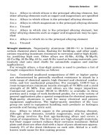
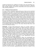
In the above equation, ᐉ is the length of the conductor (i.e., the gap sep-
arating the electrodes in Fig. (D.1), and A is the cross-sectional area of
each electrode, assuming that both electrodes have the same dimen-
sions. The ratio ᐉ/A is also called the cell constant or shape factor and
has units of m
Ϫ1
.
Molar conductivities of salts. The conductivity of a strong electrolyte
solution such as KCl decreases as the solution concentration decreas-
es. For dilute solutions, or solutions sufficiently dilute that the ionic
environment does not change significantly upon further dilution, the
conductivity should decrease as it does with concentration only
because the number of charge carriers per unit volume decreases. It is
therefore convenient to factor out the dependence upon concentration
by defining the molar conductivity ⌳ of an electrolyte [Eq. (D.5)]:
␬ϭ⌳C (D.5)
If the concentration (C) is expressed in molиm
Ϫ3
, the appropriate SI
unit for molar conductivity ⌳ is Sm
3

m
Ϫ 1
mol
Ϫ1
, or Sm
2
иmol
Ϫ1
. Other
concentration units include the molиdm
Ϫ3
, or molarity, and the
mol(kg
Ϫ1
solvent), or molality. Experimentally the value of ⌳ is found
to be independent of concentration for any electrolyte whenever the
solution is sufficiently dilute. ⌳
0
, the molar conductivity extrapolated
to infinite dilution, is characteristic only of the ions and the solvent
and is independent of ionic interactions.
The German physicist Friedrich Kohlrausch found that for dilute
solutions of strong electrolytes, extrapolation of measured values of ⌳
to infinite dilution was approximately linear when done against the
Electrochemistry Basics 1019
l
I
AC
V
Figure D.1 Schematic of a conductivity cell containing an electrolyte and two inert elec-

trodes of surface A parallel to each other and separated by distance 1.
0765162_AppD_Roberge 9/1/99 8:12 Page 1019
square root of concentration. This means that the data suggest an
equation containing an empirical coefficient B characteristic of the
electrolyte [Eq. (D.6)]:
⌳ϭ⌳
0
ϪB
͙
C
ෆ
(D.6)
Molar ionic conductivities. At infinite dilution, each ionic species pre-
sent contributes a fixed amount to the total ionic conductivity, regard-
less of the nature of any other ions present. This means that the total
conductivity of a sufficiently dilute solution is given by the sum of the
individual ionic conductivities of the i different ionic species present
[Eq. (D.7)]:
␬ϭ
Α
i
␬
i
(D.7)
It is convenient to define the molar ionic conductivity ␭ of individual
ions (i.e., the conductivity of ions carrying 1 mole of charges), in the
same manner as molar conductivity of electrolytes [Eqs. (D.8) and
(D.9)]:
␬
i

ϭ␭ C
i
(D.8)
and
␬ϭ
Α
i
␭
i
C
i
(D.9)
The molar conductivity of an electrolyte salt at sufficient dilution is
then simply the sum of the molar ionic conductivity of the ions pro-
duced by dissociation of the salt [Eq. (D.10)]:
⌳
0
ϭ
Α
i
n
i
␭
0i
(D.10)
where ⌳
0
is the molar conductivity and n
i
is the number of moles of

ions i produced by the dissociation of 1 mole of the salt.
Values of ␭
0i
, the molar ionic conductivity or, in metric units the
equivalent conductance of individual ions, can be obtained from mea-
sured values of ⌳ extrapolated to give ⌳
0
. Table D.2 contains values of
aqueous equivalent ionic conductivity for many ions found in aqueous
solutions at 25°C. It should be noted that the values in this table are
given in SI units. Values in the metric units of S
Ϫ1
иcm
2
иmol
Ϫ1
would be
larger by a factor of 10. An appropriate value for the aqueous hydro-
gen ion, for example, would be 349.99 Sиcm
2
иmol
Ϫ1
.
Because ␭
0i
is a constant characteristic only of the specific ion i in
the solvent, measurement of ␬ permits following the variation of C
i
with time. One of the main applications of the technique is to monitor
water quality in modern water purification systems. However, conduc-

1020 Appendix D
0765162_AppD_Roberge 9/1/99 8:12 Page 1020
tance measurements are inherently nonselective because all ions con-
duct ionic current in an electrolyte solution.
Transport numbers in ionic solutions. When more than one ion is present
in an electrolyte solution, it is useful to describe the fraction of the ionic
conductance due to each ionic species present. The transport number
of the individual ion t
i
, sometimes called the migration number or
transference number, is therefore defined as the fraction of the con-
ductance due to that ion [Eq. (D.11)]:
t
i
ϭ (D.11)
and, in sufficiently dilute solutions [Eq. (D.12)],
t
i
ϭ (D.12)
When the solution contains only a single electrolyte salt, the above
equation simplifies to Eq. (D.13):
t
i
ϭ (D.13)
␭
0i
ᎏ
⌳
0i
␭

0i
ᎏ
Α
i
␭
0i
␬
i
ᎏ
Α
i
␬
i
Electrochemistry Basics 1021
TABLE D.2 Values of Limiting Molar Ionic Conductivity at 25°C
Cation ␭
0
, mSиm
2
иmol
Ϫ1
Anion ␭
0
, mSиm
2
иmol
Ϫ1
H
ϩ
35.00 OH

Ϫ
19.84
1
ր
3
Al
3ϩ
6.30 Br
Ϫ
7.82
Ag
ϩ
6.19 CH
3
CO
2
Ϫ
4.09
1
ր
2
Ba
2ϩ
6.36 C
2
H
5
CO
2
Ϫ

3.58
1
ր
2
Ca
2ϩ
5.95 C
6
H
5
CO
2
Ϫ
3.24
1
ր
2
Cu
2ϩ
5.36 Cl
Ϫ
7.64
1
ր
2
Fe
2ϩ
5.40 ClO
3
Ϫ

6.46
1
ր
3
Fe
3ϩ
6.84 ClO
4
Ϫ
6.74
K
ϩ
7.35 CN
Ϫ
4.45
1
ր
3
La
3ϩ
6.97
1
ր
2
CO
3
2Ϫ
5.93
Li
ϩ

3.87 F
Ϫ
5.54
1
ր
2
Mg
2ϩ
5.30
1
ր
3
Fe(CN)
6
3 Ϫ
10.1
Na
ϩ
5.01
1
ր
4
Fe(CN)
6
4Ϫ
11.1
NH
4
ϩ
7.35 HCO

3
Ϫ
4.45
1
ր
2
Ni
2ϩ
5.30 HCO
2
Ϫ
5.46
1
ր
2
Pb
2ϩ
6.95 HSO
4
Ϫ
5.20
1
ր
2
Zn
2ϩ
5.28 I
Ϫ
7.69
MnO

4
Ϫ
6.10
NO
3
Ϫ
7.15
1
ր
3
PO
4
3 Ϫ
8.00
1
ր
2
SO
4
2 Ϫ
8.00
0765162_AppD_Roberge 9/1/99 8:12 Page 1021
Transport numbers vary with the nature of the dissolved salt and of
the solution as well as with concentration of the electrolyte. Transport
numbers do change with concentration in a solution of a single salt,
but only slightly. However, because the transport number of an ion is
the fraction of the total ionic conductance due to that ion, the trans-
port number of any particular ion or ions can be reduced to virtually
zero by the addition to the solution of a large concentration of some
salt that does not contain them. Electrochemists often make use of this

technique.
Note that the units for molar ionic conductivity, Sиm
2
иmol
Ϫ1
, are
units of velocity under a uniform potential gradient. As a consequence
these values are also referred to as limiting ionic mobility (u
i
),
expressed as Eq. (D.14):
u
i
ϭ (D.14)
leading to the following expression of conductivity [Eq. (D.15)]:
␬ϭF
Α
i
|z
i
|u
i
C
i
(D.15)
and transport number [Eq. (D.16)]:
t
i
ϭ (D.16)
where |z

i
| is the absolute valence of ion species i. Table D.3 contains
values of limiting ionic mobility corresponding to the equivalent ionic
conductivity values presented in Table D.2.
Example The conductivity of protons (H
ϩ
), a value of 0.35 Sиm
2
иmol
Ϫ1
, is
converted into a mobility value as follows:
1. 3.5 ϫ 10
Ϫ2
Sиm
2
иmol
Ϫ
ϭ 3.5 ϫ 10
Ϫ2
Aиm
2
иmol
Ϫ1
иV
Ϫ1
2. 3.5 ϫ 10
Ϫ2
Aиmиmol
Ϫ1

per V/m ϭ 3.5 ϫ 10
Ϫ2
Cиmиmol
Ϫ1
s
Ϫ1
per V/m and divid-
ing by F (C mol
Ϫ1
)
3. 3.5 ϫ 10
Ϫ2
Cиmиmol
Ϫ1
s
Ϫ1
/(96,485 C/mol) per V/m ϭ 3.6 ϫ 10
Ϫ7
m/s per V/m
Mobility of uncharged species in solution. The mobility of an uncharged
particle u
i
can be estimated by dividing its diffusion coefficient D
i
by
the product of the Boltzmann constant and the absolute temperature.
Uncharged particles are unaffected by an electric field, and their
motion is driven only by diffusion. In molar terms, this is expressed as
u
i

ϭ because Boltzmann constant ϭ
R
ᎏ
N
A
D
i
N
A
ᎏ
RT
|z
i
|u
i
C
i
ᎏᎏ
Α
i
|z
i
|u
i
C
i
␭
i
ᎏ
|z

i
|F
1022 Appendix D
0765162_AppD_Roberge 9/1/99 8:12 Page 1022
where R is the gas constant (8.314 JиK
Ϫ1
иmol
Ϫ1
) and N
A
is the Avogadro
number (6.023 ϫ 10
23
moleculesиmol
Ϫ1
).
For a particle of macroscopic dimensions moving through an ideal
hydrodynamic continuum with velocity v, this force will be opposed by
the viscous drag of the medium until these two forces are in balance.
Stokes treated the ideal case of a spherical particle moving through an
ideal hydrodynamic medium. Under these conditions Stokes’s law
gives the mobility [Eq. (D.17)]:
u
i
ϭ (D.17)
In this equation ␩ is the viscosity, sometimes called the dynamic vis-
cosity, of the medium, and r
i
is the radius of the particle. Equating
these two equations of ionic mobility gives the Stokes-Einstein equa-

tion [Eq. (D.18)]:
D
i
ϭ (D.18)
The Stokes-Einstein equation can be used to calculate the diffusion
coefficients of uncharged species. It gives reasonable results if the
RT
ᎏ
6␲␩N
A
r
i
1
ᎏ
6␲␩r
i
Electrochemistry Basics 1023
TABLE D.3 Values of Limiting Ionic Mobility at 25°C
Cation u, 10
Ϫ8
m
2
иs
Ϫ1
иV
Ϫ1
Anion u, 10
Ϫ8
m
2

иs
Ϫ1
иV
Ϫ1
H
ϩ
36.28 OH
Ϫ
20.56
Al
3ϩ
6.53 Br
Ϫ
8.10
Ag
ϩ
6.42 CH
3
CO
2
Ϫ
4.24
Ba
2ϩ
6.59 C
2
H
5
CO
2

Ϫ
3.71
Ca
2ϩ
6.17 C
6
H
5
CO
2
Ϫ
3.36
Cu
2ϩ
5.56 C1
Ϫ
7.92
Fe
2ϩ
5.60 C1O
3
Ϫ
6.70
Fe
3ϩ
7.09 C1O
4
Ϫ
6.99
K

ϩ
7.62 CN
Ϫ
4.61
La
3ϩ
7.22 CO
3
2 Ϫ
6.15
Li
ϩ
4.01 F
Ϫ
5.74
Mg
2ϩ
5.49 Fe(CN)
6
3 Ϫ
10.47
Na
ϩ
5.19 Fe(CN)
6
4 Ϫ
11.50
NH
4
ϩ

7.62 HCO
3
Ϫ
4.61
Ni
2ϩ
5.49 HCO
2
Ϫ
5.66
Pb
2ϩ
7.20 HSO
4
Ϫ
5.39
Zn
2ϩ
5.47 I
Ϫ
7.97
MnO
4
Ϫ
6.32
NO
3
Ϫ
7.41
PO

4
3 Ϫ
8.29
SO
4
2 Ϫ
8.29
0765162_AppD_Roberge 9/1/99 8:12 Page 1023
species diffusing is roughly spherical and much larger than the solvent
molecules.
Mobility of ions in solution. When an ion rather than an uncharged
species is in motion, the force upon it is determined by the interaction
of the electric field and the ionic charge. The conductivity due to a sin-
gle ion submitted to an electrical field of unity (i.e., 1 V/m), is
expressed as Eq. (D.19):
␬
i
ϭ C
i
|z
i
|u
i
F (D.19)
or as ␭
i
ϭ u
i
F because ␭
i

ϭ␬
i
/C
i
Again, remember that C
i
expresses the concentration of species i in
terms of moles of charges produced (i.e., 1 mole CaCl
2
generates 2
moles of charge). The ionic velocity v
i
is the product of ionic mobility
and the electrical field (␰) expressed in V/m [Eq. (D.20)]:
v
i
ϭ u
i
␰ (D.20)
The comparison between the mobility of ionic species and Fick’s first
law of diffusion has permitted Einstein to express the mobility of ionic
species as Eq. (D.21):
u
i
ϭ or D
i
ϭ (D.21)
or, as expressed in Nernst-Einstein equation [Eq. (D.22)]:
␭
i

ϭ (D.22)
Some care is required in its use because molar conductivity of ions
and specific ionic conductance are often given in the form ␭
i
/Z
i
, as
indicated by species such as
1
⁄
2
Ca
2ϩ
listed in Table D.2. One redundant
z
i
must then be dropped from the last equation. Alternatively, the val-
ues given in that form may be converted to those of real species, that
is ␭
0
(Ca
2ϩ
) is simply 2 ␭
0
(
1
⁄
2
Ca
2ϩ

).
New expressions of ionic mobility can be obtained [Eqs. (D.23) to
(D.25)] by combining Stokes-Einstein equation with Einstein equation:
D
i
ϭϭ (D.23)
and
u
i
ϭ (D.24)
z
i
F
ᎏᎏ
6␲␩ N
A
r
i
RTu
i
ᎏ
z
i
F
RT
ᎏ
6␲␩N
A
r
i

z
i
2
F
2
D
i
ᎏ
RT
RTu
i
ᎏ
z
i
F
z
i
FD
i
ᎏ
RT
1024 Appendix D
0765162_AppD_Roberge 9/1/99 8:12 Page 1024