Pearson survey. The Pearson survey, named after its inventor, is used
to locate coating defects in buried pipelines. Once these defects have
been identified, the protection levels afforded by the CP system can be
investigated at these critical locations in more detail.
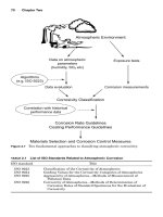
Methodology. An ac signal of around 1000 Hz is imposed onto the
pipeline by means of a transmitter, which is connected to the pipeline
and an earth spike, as shown in Fig. 11.25. Two survey operators make
earth contact either through metal studded boots or aluminum poles.
A distance of several meters typically separates the operators.
Essentially, the signal measured by the receiver is the potential gradi-
ent over the distance between the two operators. Defects are located by
a change in the potential gradient, which translates into a change in
signal intensity.
As in the CIPS technique, the measurements are usually recorded
by walking directly over the pipeline. As the front operator approaches
a defect, increasing signal intensity is recorded. As the front person
moves away from the defect, the signal intensity drops and later picks
up again as the rear operator approaches the defect. The interpreta-
tion of signals can obviously become confusing when several defects
are located between the two operators. In this case, only one person
walks directly over the pipeline, with the connecting leads at a right
angle to the pipeline.
In principle, a Pearson survey can be performed with an impressed
cathodic protection system remaining energized. Sacrificial anodes
Cathodic Protection 913
Buried pipeline
Earth
spike
Test station
Receiver
Aluminum

pole
X
(
(
(
Signal emitted at defect
Coating defect
Transmitter
Figure 11.25 Pearson survey methodology (schematic).
0765162_Ch11_Roberge 9/1/99 6:37 Page 913
should be disconnected because the signal from these may otherwise
mask actual coating defects. A three-person team is usually required
to locate the pipeline, perform the survey measurements, place defect
markers into the ground, and move the transmitters periodically. The
operator carrying the receiver should be highly experienced, especially
if the survey is based on audible signals and instrument sensitivity
settings. Under these conditions, the results are completely dependent
on this operator’s judgment.
Advantages and limitations. By walking the entire length of the
pipeline, an overall inspection of the right-of-way can be made together
with the measurements. In principle, all significant defects and metal-
lic conductors causing a potential gradient will be detected. There are
no trailing wires and the impressed CP current does not have to be
pulsed.
The disadvantages are similar to those of CIPS because the entire
pipeline has to be walked and contact established with ground. The
technique is therefore unsuitable to roads, paved areas, rivers, and so
forth. Fundamentally, no severity of corrosion damage is indicated and
no direct measure of the performance of the CP system is obtained.
The survey results can be very operator dependent, if no automated

signal recording is performed.
Direct current voltage gradient (DCVG) surveys. DCVG surveys are a
more recent methodology to locate defects on coated buried pipelines
and to make an assessment of their severity. The technique again
relies on the fundamental effect of a potential gradient being estab-
lished in the soil at coating defects under the application of CP cur-
rent; in general, the greater the size of the defect, the greater the
potential gradient. The DCVG data is intricately tied to the overall
performance of a CP system, because it gives an indication of current
flow and its direction in the soil.
Methodology. The potential gradient is measured by an operator
between two reference electrodes (usually of the saturated Cu/CuSO
4
type), separated by a distance of say half a meter. The appearance of
these electrodes resembles a pair of cross-country ski poles (Fig.
11.26). A pulsed dc signal is imposed on the pipeline for DCVG mea-
surements. The pulsed input signal minimizes interference from other
current sources (other CP systems, electrified rail transit lines, telluric
effects). This signal can be obtained with an interrupter on an existing
rectifier or through a secondary current pulse superimposed on the
existing “steady” CP current.
The operator walking the pipeline observes the needle of a milli-
voltmeter needle to identify defect locations. (More recently devel-
914 Chapter Eleven
0765162_Ch11_Roberge 9/1/99 6:37 Page 914
oped DCVG systems are digital and do not have a needle as such.)
It is preferable for the operator to walk directly over the pipeline,
but it is not strictly necessary. The presence of a defect is indicated
by a increased needle deflection as the defect is approached, no nee-
dle deflection when the operator is immediately above the defect,

and a decreasing needle deflection as the operator walks away from
the defect (Fig. 11.27). It is claimed that defects can be located with
an accuracy of 0.1 to 0.2 m, which represents a major advantage in
minimizing the work of subsequent digs when corrective action has
to be taken.
Cathodic Protection 915
Figure 11.26 DCVG measuring equipment. (Courtesy of CSIR
North America Inc.)
0765162_Ch11_Roberge 9/1/99 6:37 Page 915
An additional feature of the DCVG technique is that defects can be
assigned an approximate size factor. Sizing is most important for iden-
tifying the most critical defects and prioritizing repairs. Leeds and
Grapiglia
15
have provided details on the sizing procedure. An empiri-
cally based rating based on the so-called %IR value has been adopted
in general terms as follows:
■
0 to 15%IR (“small”): No repair required usually.
■
16 to 35%IR (“medium”): Repairs may be recommended.
■
36 to 60%IR (“large”): Early repair is recommended.
■
61 to 100%IR (“extra large”): Immediate repair is recommended.
To establish a theoretical basis for the %IR value, the pipeline poten-
tial measured relative to remote earth at a test post must be consid-
ered. This potential (V
t
) is made up of two components:

916 Chapter Eleven
Increasing signal
strength (when
approaching defect)
Needle deflection
points toward
defect
Needle deflection
points toward
defect
No needle deflection
Buried pipeline
Decreasing signal
strength (when
leaving defect)
No signal
(when directly
above defect)
X
X
Location of coating defect
Equipotential lines
Figure 11.27 DCVG methodology (schematic).
0765162_Ch11_Roberge 9/1/99 6:37 Page 916
V
t
ϭ V
i
ϩ V
s

where V
i
is the voltage across the pipe to soil interface and V
s
is the
voltage between the soil surrounding the pipe and remote earth. The
%IR value is defined as
%IR ϭ
Essentially the pipe-to-soil interface and the soil between the pipe
and remote earth can be viewed as two resistors in series, with a
potential difference across each of them. Although V
i
cannot be mea-
sured easily in practice, V
s
can be measured relatively easily with the
DCVG instrumentation (one reference electrode is initially placed at
the defect epicenter, and the voltage change is then summed as the
electrodes are moved away from the epicenter to remote earth). In
practice, the V
s
value measured at a test post has to be extrapolated to
a value at the defect location. Two test post readings bracketing the
defect location and simple linear extrapolation are usually employed.
For effective protection of the defect by the CP system, the V
s
/V
t
ratio
should be small. The overall shift in pipeline potential due to the appli-

cation of CP should be manifested by mainly shifting V
i
, not V
s
. Higher
%IR values imply a lower level of cathodic protection.
Because the DCVG technique can be used to determine the direction
of current flow in the soil, a further defect severity ranking has been
proposed. As indicated in Fig. 11.1, current will tend to flow to a defect
under the protective influence of the CP system. Corrosion damage
(anodic dissolution) at the defect has an opposite influence; it will tend
to make current flow away from the defect. Using an adaptation of the
DCVG technique, it has been claimed that it is possible to establish
whether current flows to or from a defect, with the CP system switched
ON and OFF in a pulsed cycle.
Advantages and limitations. Fundamentally, the DCVG technique is
particularly suited to complex CP systems in areas with a relatively
high density of buried structures. These are generally the most diffi-
cult survey conditions. The DCVG equipment is relatively simple and
involves no trailing wires. Although a severity level can be identified
for coating defects, the rating system is empirical and does not provide
quantitative kinetic corrosion information. The survey team’s rate of
progress is dependent on the number of coating defects present.
Terrain restrictions are similar to the CIPS technique. However, it
may be possible to place the electrode tips in asphalt or concrete sur-
face cracks or in between the gaps of paving stones.
V
s
ᎏ
V

t
Cathodic Protection 917
0765162_Ch11_Roberge 9/1/99 6:37 Page 917
Corrosion coupons. Corrosion coupons connected to cathodically pro-
tected structures are finding increasing application for performance
monitoring of the CP system. Essentially these coupons, installed
uncoated, represent a defect simulation on the pipeline under con-
trolled conditions. These coupons can be connected to the pipeline via
a test post outlet, facilitating a number of measurements such as
potential and current flow.
A publication describing an extensive coupon development and mon-
itoring program on the Trans Alaska Pipeline System
16
serves as an
excellent case study. This coupon monitoring program was designed to
assess the adequacy of the CP system under conditions where tech-
niques involving CP current interruption on the pipeline were imprac-
tical. Although the coupon monitoring methodology is based on
relatively simple principles, significant development efforts and atten-
tion to detail are typically required in practice, as this case study
amply illustrates.
Methodology. Perhaps the most important consideration in the
installation of corrosion coupons is that a coupon must be representa-
tive of the actual pipeline surface and defect. The exact metallurgical
detail and surface finish as found on the actual pipeline are therefore
required on the coupon. The influence of corrosion product buildup
may also be important. Furthermore the environmental conditions of
the coupon and the pipe should also be matched (temperature, soil con-
ditions, soil compaction, oxygen concentration, etc.). Current shielding
effects on the bonded coupon should be avoided.

Several measurements can be made after a coupon-type corrosion
sensor has been attached to a cathodically protected pipeline.
17
ON
potentials measured on the coupon are in principle more accurate than
those measured on a buried pipe, if a suitable reference electrode is
installed in close proximity to the coupon. The potentials recorded with
a coupon sensor may still contain a significant IR drop error, but this
error is lower than that of surface ON potential measurements. Instant-
OFF potentials can be measured conveniently by interrupting the
coupon bond wire at a test post. Similarly, longer-term depolarization
measurements can be performed on the coupon without depolarizing
the entire buried structure. Measurement of current flow to or from the
coupon and its direction can also be determined, for example, by using
a shunt resistor in the bond wire. Importantly, it is also possible to
determine corrosion rates from the coupon. Electrical resistance sen-
sors provide an option for in situ corrosion rate measurements as an
alternative to weight loss coupons.
The surface area of the coupon used for monitoring is an important
variable. Both the current density and the potential of the coupon are
918 Chapter Eleven
0765162_Ch11_Roberge 9/1/99 6:37 Page 918
dependent on the area. In turn, these two parameters have a direct
relation to the kinetics of corrosion reactions.
Advantages and limitations. A number of important corrosion parame-
ters can be conveniently monitored under controlled conditions, with-
out any adjustments to the energized CP system of the structure. The
measurement principles are relatively simple. It is difficult (virtually
impossible) to guarantee that the coupon will be completely represen-
tative of an actual defect on a buried structure. The measurements are

limited to specific locations. The coupon sensors have to be extremely
robust and relatively simple devices to perform satisfactorily under
field conditions.
References
1. Ashworth, V., The Theory of Cathodic Protection and Its Relation to the
Electrochemical Theory of Corrosion, in Ashworth, V., and Booker, C. J. L. (eds.),
Cathodic Protection, Chichester, U.K., Ellis Horwood, 1986.
2. Peabody, A. W., Control of Pipeline Corrosion, Houston, Tex., NACE International,
1967.
3. Eliassen, S., and Holstad-Pettersen, N., Fabrication and Installation of Anodes for
Deep Water Pipelines Cathodic Protection, Materials Performance, 36(6):20–23
(1997).
4. Sydberger, T., Edwards, J. D., and Tiller, I. B., Conservatism in Cathodic Protection
Designs, Materials Performance, 36(2):27–32 (1997).
5. Shreir, L. L., and Hayfield, P. C. S., Impressed Current Anodes, in Ashworth, V., and
Booker, C. J. L. (eds.) Cathodic Protection, Chichester, U.K., Ellis Horwood, 1986.
6. Shreir, L. L., Jarman, R. A., and Burstein, G. T. (eds.), Corrosion, vol. 2, 3d ed.,
Oxford, Butterworth Heinemann, 1994.
7. Beavers, J. A., and Thompson, N. G., Corrosion Beneath Disbonded Pipeline
Coatings, Materials Performance, 36(4):13–19, (1997).
8. Jack, T. R., Wilmott, M. J., and Sutherby, R. L., Indicator Minerals Formed During
External Corrosion of Line Pipe, Materials Performance, 34(11):19–22 (1995).
9. Kirkpatrick, E. L., Basic Concepts of Induced AC Voltages on Pipelines, Materials
Performance, 34(7):14–18 (1995).
10. Allen, M. D., and Ames, D. W., Interaction and Stray Current Effects on Buried
Pipelines: Six Case Histories, in Ashworth, V., and Booker, C. J. L. (eds.), Cathodic
Protection Chicester, U.K., Ellis Horwood, 1986, pp. 327–343.
11. NACE International and Institute of Corrosion, Cathode Protection Monitoring for
Buried Pipelines, pub. no. CEA 54276, Houston, Tex, NACE International, 1988.
12. Goloby, M. V., Cathodic Protection on the Information Superhighway, Materials

Performance, 34(7):19–21 (1995).
13. Pawson, R. L., Close Interval Potential Surveys—Planning, Execution, Results,
Materials Performance, 37(2):16–21 (1998).
14. NACE International, Specialized Surveys for Buried Pipelines, pub. no. 54277,
Houston, Tex, NACE International, 1990.
15. Leeds, J. M., and Grapiglia, J., The DC Voltage-Gradient Method for Accurate
Delineation of Coating Defects on Buried Pipelines, Corrosion Prevention and
Control,42(4):77–86 (1995).
16. Stears, C. D., Moghissi, O. C., and Bone, III, L., Use of Coupons to Monitor Cathodic
Protection of an Underground Pipeline, Materials Performance, 37(2):23–31 (1998).
17. Turnipseed, S. P., and Nekoksa, G., Potential Measurement on Cathodically
Protected Structures Using an Integrated Salt Bridge and Steel Ring Coupon,
Materials Performance, 35(6):21–25 (1996).
Cathodic Protection 919
0765162_Ch11_Roberge 9/1/99 6:37 Page 919
921
Anodic Protection
12.1 Introduction 921
12.2 Passivity of Metals 923
12.3 Equipment Required for Anodic Protection 927
12.3.1 Cathode 929
12.3.2 Reference electrode 929
12.3.3 Potential control and power supply 930
12.4 Design Concerns 930
12.5 Applications 932
12.6 Practical Example: Anodic Protection in the Pulp and
Paper Industry 933
References 938
12.1 Introduction
In contrast to cathodic protection, anodic protection is relatively new.

Edeleanu first demonstrated the feasibility of anodic protection in 1954
and tested it on small-scale stainless steel boilers used for sulfuric acid
solutions. This was probably the first industrial application, although
other experimental work had been carried out elsewhere.
1
This tech-
nique was developed using electrode kinetics principles and is some-
what difficult to describe without introducing advanced concepts of
electrochemical theory. Simply, anodic protection is based on the for-
mation of a protective film on metals by externally applied anodic cur-
rents. Anodic protection possesses unique advantages. For example,
the applied current is usually equal to the corrosion rate of the pro-
tected system. Thus, anodic protection not only protects but also offers
a direct means for monitoring the corrosion rate of a system. As an
Chapter
12
0765162_Ch12_Roberge 9/1/99 6:40 Page 921
enthusiast and famous corrosion engineer claimed, “anodic protection
can be classed as one of the most significant advances in the entire his-
tory of corrosion science.”
2
Anodic protection can decrease corrosion rate substantially. Table 12.1
lists the corrosion rates of austenitic stainless steel in sulfuric acid solu-
tions containing chloride ions with and without anodic protection.
Examination of the table shows that anodic protection causes a 100,000-
fold decrease in corrosive attack in some systems. The primary advan-
tages of anodic protection are its applicability in extremely corrosive
environments and its low current requirements.
2
Table 12.2 lists several

systems where anodic protection has been applied successfully.
Anodic protection has been most extensively applied to protect equip-
ment used to store and handle sulfuric acid. Sales of anodically pro-
tected heat exchangers used to cool H
2
SO
4
manufacturing plants have
represented one of the more successful ventures for this technology.
922 Chapter Twelve
TABLE 12.1 Anodic Protection of S30400 Stainless Steel Exposed to
an Aerated Sulfuric Acid Environment at 30°C with and without
Protection at 0.500 V vs. SCE
Corrosion rate, ␮m
и
y
-1
Acid concentration, M NaCl, M Unprotected Protected
0.5 10
Ϫ5
360 0.64
0.5 10
Ϫ3
74 1.1
0.5 10
Ϫ1
81 5.1
510
Ϫ5
49,000 0.41

510
Ϫ3
29,000 1.0
510
Ϫ1
2,000 5.3
TABLE 12.2 Current Requirements for Anodic Protection
Current density
To passivate, To maintain,
H
2
SO Temperature, °C Alloy mAиcm
Ϫ2
␮Aиcm
Ϫ2
1 M 24 S31600 2.3 12
15% 24 S30400 0.42 72
30% 24 S30400 0.54 24
45% 65 S30400 180 890
67% 24 S30400 5.1 3.9
67% 24 S31600 0.51 0.10
67% 24 N08020 0.43 0.9
93% 24 Mild steel 0.28 23
99.9% (oleum) 24 Mild steel 4.7 12
H
3
PO
4
75% 24 Mild steel 41 20,000
115% 82 S30400 3.2 ϫ 10

Ϫ5
1.5 ϫ 10
Ϫ4
NaOH
20% 24 S30400 4.7 10
0765162_Ch12_Roberge 9/1/99 6:40 Page 922
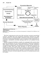
Among the parameters that are particularly affected by sensitization
are i
p
and i
cc
, as defined in Fig. 12.1. In this example, the ability to sus-
tain passivity increases as the current density to maintain passivity
(i
p
) decreases and as the total film resistance increases, as indicated
from measurements obtained with different metals exposed to 67%
sulfuric acid (Table 12.3). The lower or more reducing the potential at
which a passive metal becomes active, the greater the stability of pas-
sivity. The depassivation potential corresponding to the passive-active
transition, called the Flade potential, can differ appreciably from E
pp
measured by going through the active-passive process of the same sys-
tem. This technical distinction is important for the control aspect of
anodic protection where E
pp
is the potential to traverse to obtain pas-
sivation, and the Flade potential is the potential to avoid traversing
back into active corrosion.
Passivity can also be readily produced in the absence of an externally

applied passivating potential by using oxidants to control the redox
potential of the environment. Very few metals will passivate in nonoxi-
dizing acids or environments, when the redox potential is more cathodic
than the potential at which hydrogen can be produced. A good example
of that behavior is titanium and some of its alloys, which can be readily
passivated by most acids, whereas mild steel requires a strong oxidizing
924 Chapter Twelve
Potential
Log (Current density)
E
corr

(corrosion potential)
i
p
(passive current)
Oxygen evolution
i
cc
(critical current)
active
E
pp
(passivation
potential)
transpassive
passive
Figure 12.1 Hypothetical polarization diagram for a passivable system with active, pas-
sive, and transpassive regions.
0765162_Ch12_Roberge 9/1/99 6:40 Page 924

agent, such as fuming HNO
3
, for its passivation. Alloying with a more
easily passivated metal normally increases the ease of passivation and
lowers the passivation potential, as in the alloying of iron and chromium
in 10% sulfuric acid (Table 12.4). Small additions of copper in carbon
steels have been found to reduce i
p
in sulfuric acid. Each alloy system has
to be evaluated for its own passivating behavior, as illustrated by the
case Ni-Cr alloys where both the additions of nickel to chromium and
chromium to nickel decrease the critical current density in a mixture
of sulfuric acid and 0.25 M K
2
SO
4
(Table 12.5).
1
The parameters defining and controlling the passivation domain of
a system are thus directly related to the composition, concentration,
purity, temperature, and agitation of the environment. This is illus-
trated with the current densities required to obtain passivity (i
cc
), and
to maintain passivity (i
p
), for a S30400 steel in different electrolytes,
as presented in Table 12.6. From the data in this table, it can be seen
that it is approximately 100,000 times easier to passivate large areas
of this steel in contact with 115% phosphoric acid than in 20% sodium

hydroxide. The concentration of the electrolyte is also important, and
for a S31600 steel in sulfuric acid, although there is a maximum cor-
rosion rate at about 55%, the critical current density decreases pro-
gressively as the concentration of acid increases (Table 12.7).
1
Anodic Protection 925
-150
50
-2-1012345
250
450
650
850
1050
1250
Log Current density (µA cm
-2
)
Potential (mV vs. SHE)
No sensitization
0.3 h
1 h
1000 h
Figure 12.2 Anodic polarization curves of S30400 steel in a 1 M H
2
SO
4
at 90°C after sen-
sitization for various times.
0765162_Ch12_Roberge 9/1/99 6:40 Page 925

The presence in the environment of impurities that retard the for-
mation of a passive film or accelerate its degradation is often detri-
mental. In this context, chloride ions can be quite aggressive for
many alloys and particularly for steels and stainless steels. As an
example, the addition of 3% HCl hydrochloric acid to 67% sulfuric
acid raises the critical current density for the passivation of a S31600
stainless steel from 0.7 to 40 mAиcm
Ϫ2
and the current density to
maintain passivity from 0.1 to 60 ␮Aиcm
Ϫ2
. Therefore, the use of the
calomel electrode in anodic-protection systems is not recommended
because of the possible leakage of chloride ions into the electrolyte,
926 Chapter Twelve
TABLE 12.3 Current Density to Maintain Passivity and Film
Resistance of Some Metals in 67% Sulfuric Acid
Metal or alloy i
p
, ␮Aиcm
Ϫ2
Film resistance, M⍀иcm
Mild steel 150 0.026
S30400 steel 2.2 0.50
S31000 steel 0.5 2.1
S31600 steel 0.1 17.5
Titanium 0.08 1.75
N08020 0.03 4.6
TABLE 12.4 Effect on Critical Current Density
and Passivation Potential of Chromium Content

for Iron-Chromium Alloys in 10% Sulfuric Acid
Chromium, % i
cc
, mAиcm
Ϫ2
E
pp
, V vs. SHE
0 1000 ϩ0.58
2.8 360 ϩ0.58
6.7 340 ϩ0.35
9.5 27 ϩ0.15
14.0 19 Ϫ0.03
TABLE 12.5 Effect on Critical Current Density and
Passivation Potential on Alloying Nickel with Chromium
in 0.5 M and 5 M H
2
SO
4
Containing 0.25 M K
2
SO
4
Ni, % i
cc
, mAиcm
Ϫ2
E
pp
, V vs. SHE

0.5 M 5 M 0.5 M 5 M
100 100 23 ϩ0.36 ϩ0.47
91 0.95 3.9 ϩ0.06 ϩ0.14
77 0.11 0.82 ϩ0.07 ϩ0.08
49 0.020 0.20 ϩ0.03 ϩ0.06
27 0.012 0.041 ϩ0.02 ϩ0.05
10 0.0013 0.011 ϩ0.04 ϩ0.08
1 1.0 5.0 Ϫ0.32 Ϫ0.20
0 1.5 8.0 Ϫ0.30 Ϫ0.20
0765162_Ch12_Roberge 9/1/99 6:40 Page 926
-1000
-500
0
500
1000
1500
2000
22
°
C
60
°
C
-2.00 2.00 2.50-1.50 1.50-1.00 1.00-0.50 0.500.00
Log Current density (mA cm
-2
)
Potential (mV vs. SHE)
Figure 12.3 Forward and backward potentiostatic anodic polarization curves for mild
steel in 10% sulfuric acid at 22 and 60°C.

Sulfuric acid
Power
supply
Hastelloy
cathode
Hg/HgSO4
reference electrode
Figure 12.4 Schematic of an anodic protection system for a sulfuric acid storage vessel.
0765162_Ch12_Roberge 9/1/99 6:40 Page 928
equipment to be protected, considering any special operational condi-
tions. As described earlier, the electrochemical parameters of concern
are the potential at which the vessel must be maintained for corrosion
protection, the current required to establish passivity, and the current
required to maintain passivity. The electrode potential can be deter-
mined directly from polarization curves, and the required currents can
be estimated from the polarization data. However, because the current
is so strongly time dependent, its variations with respect to time must
be carefully estimated. Empirical data available from field installations
are the best source for this type of information.
3
Special care and attention should also be focused on estimating the
solution resistivity of a system because it is important in determining
the overall circuit resistance. The power requirements for the dc power
supply should be as low as possible to reduce operating costs. The
solution resistivity should usually be sufficiently low so that the cir-
cuit resistance is controlled by the cathode surface area. It is essen-
tial for a system to have good throwing power or good ability for the
applied current to reach the required value over complex geometry
and variable distances. In general, a uniform distribution of potential
over a regular-shaped passivated surface can be readily obtained by

anodic protection. It is much more difficult to protect surface irregu-
larities, such as the recessions around sharp slots, grooves, or crevices
because the required current density will not be obtained in these
areas. This incomplete passivation can have catastrophic conse-
quences. This difficulty can be overcome by designing the surface to
avoid these irregularities or by using a metal or alloy that is easily
passivated with as low a critical current density as possible. In the
rayon industry, crevice corrosion in titanium has been overcome by
alloying it with 0.1% palladium.
1
The actual passivation of a surface is very rapid if the applied cur-
rent density is greater than the critical value. However, because of the
high current requirements, it has been found to be neither technically
nor economically practical to passivate the whole surface of a large
vessel in the same initial period. For a storage vessel with an area of
1000 m
2
, for example, a current of 5000 A could be necessary. It is
therefore essential to avoid these very high currents by using one of a
few techniques. It may be possible and practical, for example, to lower
the temperature of the electrolyte, thereby reducing the critical cur-
rent density before passivating the metal. If a vessel has a very small
floor area, it may be treated in a stepwise manner by passivating the
base, then the lower areas of the walls, and finally the upper areas of
the walls, but this technique is not practical for very large storage
tanks with a considerable floor area.
1
Another method that has been successful is to passivate the metal by
using a solution with a low critical current density (such as phosphoric
Anodic Protection 931

0765162_Ch12_Roberge 9/1/99 6:40 Page 931
sive). A potentiodynamic curve of each of these types of behavior is
shown, respectively, in Figs. 12.6 through 12.9. Astable behavior occurs
infrequently because it requires a single anodic-cathodic intersection
on the negative resistance portion of the anodic curve. This is an unsta-
ble operating condition that results in continuous oscillations between
active and passive potentials. Various alloys in elevated temperature
sulfuric acid are known to exhibit such behavior.
6
The four types of mixed potential models presented in Figs. 12.6 to
12.9 are simplistic and do not necessarily reflect the complete behav-
ior of carbon steel in Kraft liquors because the models all assume some
sort of steady states. Figure 12.10 depicts typical curves from an in
situ test in a white liquor clarifier at different scan rates. The passive
state does not exist until after the active-passive transition is tra-
versed. Therefore, unless sufficient anodic current density is dis-
charged from carbon steel by a naturally occurring cathodic reaction or
an applied anodic protection current, the carbon steel liquor interface
remains monostable (active) because the passive film and its low cur-
rent density properties do not exist.
Under normal operating chemistries in white and green Kraft
liquors, carbon steel exhibits a monostable (active) behavior, and the
bistable behavior occurs only after the passivation process has reached
some degree of completion, as predicted by Tromans and verified by
934 Chapter Twelve
-100
100
200
300
Bistable

Anodic curve
Astable
Monostable active
Monostable passive
-200
-300
0
-3 -2.5 -2 -1.5 -1 -0.5 0 0.5 1
Log current density (mA cm
-2
)
Potential (V vs. SSE)
Figure 12.5 Possible combinations of anodic/cathodic intersections in the mixed poten-
tial representation of carbon steel exposed to Kraft liquors.
0765162_Ch12_Roberge 9/1/99 6:40 Page 934
Anodic Protection 935
-100
100
200
300
-200
-300
0
-3 -2.5 -2 -1.5 -1 -0.5 0 0.5 1
Log current density (mA cm
-2
)
Potential (V vs. SSE)
Figure 12.6 Theoretical polarization curve illustrating the monostable (active) behavior
of mild steel exposed to Kraft liquors.

-100
100
200
300
-200
-300
0
-3 -2.5 -2 -1.5 -1 -0.5 0 0.5 1
Log current density (mA cm
-2
)
Potential (V vs. SSE)
Figure 12.7 Theoretical polarization curve illustrating the bistable behavior of mild steel
exposed to Kraft liquors.
0765162_Ch12_Roberge 9/1/99 6:40 Page 935
936 Chapter Twelve
-100
100
200
300
-200
-300
0
-3 -2.5 -2 -1.5 -1 -0.5 0 0.5 1
Log current density (mA cm
-2
)
Potential (V vs. SSE)
Figure 12.8 Theoretical polarization curve illustrating the monostable (passive) behav-
ior of mild steel exposed to Kraft liquors.

-100
100
200
300
-200
-300
0
-3 -2.5 -2 -1.5 -1 -0.5 0 0.5 1
Log current density (mA cm
-2
)
Potential (V vs. SSE)
Figure 12.9 Theoretical polarization curve illustrating the astable behavior of mild steel
exposed to Kraft liquors.
0765162_Ch12_Roberge 9/1/99 6:40 Page 936
typical curves. However, once created, the passive state is not perma-
nently stable. When the direction of the curve is reversed, a second
stable equilibrium potential is established. During traverse of the
active-passive transition, the corrosion rate has been measured to be
only 10 percent of the total Faradaic equivalent; hence 90 percent of
the current is consumed in sulfide oxidation. Design of the protection
and control systems now incorporates all of the features required to
passivate the tank, maintain passivation, detect active areas, and
repassivate if required.
6
Some of these features are
6
1. The location of cathodes. Design is based on primary current
distribution with the ratio of the minimum to maximum current den-
sity around the circumference of the tank greater than 0.9.

2. Fluctuating liquor level. This requires higher initial current
density and more frequent repassivation cycles to form a tenacious
passive layer. When immersed, the wet/dry zone of a tank exhibits a
more positive potential than the remainder of tank, which may
account for the higher corrosion rates there. However, it has been
observed that the wet/dry zone does not get covered with surface
buildup or deposits. The constantly immersed zone builds a thick sur-
face deposit on these protected surfaces.
3. Control scheme. Conventional control schemes rely on a simple
proportional, integral algorithm (PI). This technique is not optimal
when active and passive areas exist simultaneously. The use of this
Anodic Protection 937
-100
100
200
300
-200
-300
0
-3 -2.5 -2 -1.5 -1 -0.5 0 0.5 1
Log current density (mA cm
-2
)
Potential (V vs. SSE)
0.02 mV s
-1
1 mV s
-1
Figure 12.10 Typical in situ polarization curves of carbon steel immersed in white liquor
at two scan rates.

0765162_Ch12_Roberge 9/1/99 6:40 Page 937
939
SI Units Conversion Table
How to Read This Table
The table provides conversion factors to SI units. These factors can be
considered as unity multipliers. For example,
Length: m/X
0.0254 in
0.3048 ft
means that
1 ϭ 0.0254 (m/in)
1 ϭ 0.3048 m/ft
and similarly,
1 ϭ 418.7 (W/m) / (cal/s и cm)
The SI units are listed immediately after the quantity; in this case,
length: m/X. The m stands for meter, and the X designates the non-SI
units for the same quantity. These non-SI units follow the numerical
conversion factors.
Note: In the following table at all locations, ton refers to U.S. rather
than metric ton.
Acceleration: (m/s
2
)/X 0.01 cm/s
2
7.716E-08 m/h
2
0.3048 ft/s
2
8.47E-05 ft/min
2

2.35E-08 ft/h
2
Acceleration, angular: (rad/s
2
)/X 2.78E-04 rad/min
2
7.72E ϩ 08 rad/h
2
1.74E-03 rev/min
2
APPENDIX
A
0765162_AppA_Roberge 9/1/99 6:42 Page 939
Area: m
2
/X 1.0E-04 cm
2
1.0E-12 ␮m
2
0.0929 ft
2
6.452E-04 in
2
0.8361 yd
2
4,047 acre
2.59E ϩ 06 mi
2
Current: A/X 10.0 abampere
3.3356E-10 statampere

Density: (kg/m
3
)/X 1000.0 g/cm
3
16.02 lbm/ft
3
119.8 lbm/gal
27,700 lbm/in
3
2.289E-3 grain/ft
3
Diffusion coefficient: (m
2
/s)/X 1.0E-04 cm
2
/s
2.78E-04 m
2
/h
0.0929 ft
2
/s
2.58E-05 ft
2
/h
Electrical capacitance: F/X 1A
2
иs
4
/kgиm

2
1Aиs/V
1.0E ϩ 09 abfarad
1.113E-12 statfarad
3.28 V/ft
Electric charge: C/X 1Aиs
10 abcoulomb
3.336E-10 statcoulomb
Electrical conductance: S/X 1 ⍀
Ϫ1
Electric field strength: (V/m)/X 1kgиm/Aиs
3
100 V/cm
1.0E-08 abvolt/m
299.8 statvolt/m
39.4 V/in
Electrical resistivity: (Vиm/A)/X, (⍀иm)/X 1 kgиm
3
/A
2
иs
3
1kgиm
5
/A
2
иs
3
1.0E-09 abohmиm
8.988E ϩ 11 statohmиm

Energy: J/X 3.6E ϩ 06 kWh
4.187 cal
4187 kcal
1.0E-07 erg
1.356 ftиlbf
1055 Btu
0.04214 ftиpdl
2.685E ϩ 06 hpиh
1.055E ϩ 08 therm
0.113 inиlbf
4.48E ϩ 04 hpиmin
745.8 hpиs
940 Appendix A
0765162_AppA_Roberge 9/1/99 6:42 Page 940
Energy density: (J/m
3
)/X 3.6E ϩ 06 kWh/m
3
4.187E ϩ 06 cal/cm
3
4.187E ϩ 09 kcal/cm
3
0.1 erg/cm
3
47.9 ftиlbf/ft
3
3.73E ϩ 04 Btu/ft
3
1.271E ϩ 08 kWh/ft
3

9.48E ϩ 07 hpиh/ft
3
Energy, linear: (J/m)/X 418.7 cal/cm
4.187E ϩ 05 kcal/cm
1.0E-05 erg/cm
4.449 ftиlbf/ft
3461 Btu/ft
8.81E ϩ 06 hpиh/ft
1.18E ϩ 07 kWh/ft
Energy per area: (J/m
2
)/X 41,868 cal/cm
2
4.187E ϩ 07 kcal/cm
2
0.001 erg/cm
2
14.60 ftиlbf/ft
2
11,360 Btu/ft
2
2.89E ϩ 07 hpиh/ft
2
3.87E ϩ 07 kWh/ft
2
Flow rate, mass: (kg/s)/X 1.0E-03 g/s
2.78E-04 kg/h
0.4536 lbm/s
7.56E-03 lbm/min
1.26E-04 lbm/h

Flow rate, mass/force: (kg/Nиs)/X 9.869E-05 g/cm
2
иatmиs
1.339E-08 lbm/ft
2
иatmиh
Flow rate, mass/volume: (kg/m
3
иs)/X 1000 g/cm
3
иs
16.67 g/cm
3
иmin
0.2778 g/cm
3
иh
16.02 lbm/ft
3
иs
0.267 lbm/ft
3
иmin
4.45E-03 lbm/ft
3
иh
Flow rate, volume: (m
3
/s)/X 1.0E-06 cm
3

/s
0.02832 ft
3
/s (cfs)
1.639E-05 in
3
/s
4.72E-04 ft
3
/min (cfm)
7.87E-06 ft
3
/h (cfh)
3.785E-03 gal/s
6.308E-05 gal/min (gpm)
1.051E-06 gal/h (gph)
Flux, mass: (kg/m
2
иs)/X 10 g/cm
2
иs
1.667E-05 g/m
2
иmin
2.78E-07 g/m
2
иh
4.883 lbm/ft
2
иs

0.0814 lbm/ft
2
иmin
1.356E-03 lbm/ft
2
иh
SI Units Conversion Table 941
0765162_AppA_Roberge 9/1/99 6:42 Page 941
Force: N/X 1.0E-05 dyn
1kgиm/s
9.8067 kg(force)
9.807E-03 g(force)
0.1383 pdl
4.448 lbf
4448 kip
8896 ton(force)
Force, body: (N/m
3
)/X 10 dyn/cm
3
9.807E ϩ 06 kg(f)/cm
3
157.1 lbf/ft
3
2.71E ϩ 05 lbf/in
3
3.14E ϩ 05 ton(f)/ft
3
Force per mass: (N/kg)/X 0.01 dyn/g
9.807 kg(f)/kg

9.807 lbf/lbm
0.3049 lbf/slug
Heat transfer coefficient: (W/mиK)/X 41,868 cal/sиcm
2
и°C
1.163 kcal/hиm
2
и°C
1.0E-03 erg/sиcm
2
и°C
5.679 Btu/hиft
2
и°F
12.52 kcal/hиft
2
и°C
Henry’s constant: (N/m
2
)/X 1.01326E ϩ 05 atm
133.3 mmHg
6893 lbf/in
2
47.89 lbf/ft
2
Inductance: H/X 1kgиm
2
/A
2
иs

2
1Vиs/A
1.0E-09 abhenry
8.988E ϩ 11 stathenry
Length: m/X 0.01 cm
1.0E-06 ␮m
1.0E-10 Å
0.3048 ft
0.0254 in
0.9144 yd
1609.3 mi
Magnetic flux: Wb/X 1kgиm
2
/Aиs
2
1Vиs
Mass: kg/X 1.0E-03 g
0.4536 lbm
6.48E-05 grain
0.2835 oz (avdp)
907.2 ton (U.S.)
14.59 slug
Mass per area: (kg/m
2
)/X 10 g/cm
2
4.883 lbm/ft
2
703.0 lbm/in
2

3.5E-04 ton/mi
2
942 Appendix A
0765162_AppA_Roberge 9/1/99 6:42 Page 942
Moment inertia, area: m
4
/X 1.0E-08 cm
4
4.16E-07 in
4
8.63E-03 ft
4
Moment inertia, mass: (kgиm
2
)/X 1.0E-07 gиcm
2
0.04214 lbmиft
2
1.355 lbfиftиs
2
2.93E-04 lbmиin
2
0.11 lbfиin/s
Momentum: (kgиm/s)/X 1.0E-05 gиcm/s
0.1383 lbmиft/s
2.30E-03 lbmиft/min
Momentum, angular: (kgиm
2
/s)/X 1.0E-07 gиcm
2

/s
0.04215 lbmиft
2
/s
7.02E-04 lbmиft
2
/min
Momentum flow rate: (kgиm/s
2
)/X 1.0E-05 gиcm/s
2
0.1383 lbmиft/s
2
3.84E-05 lbmиft/min
2
Power: W/X 4.187 cal/s
4187 kcal/s
1.0E-07 erg/s
1.356 ftиlbf/s
0.293 Btu/h
1055 Btu/s
745.8 hp
0.04214 ftиpdl/s
0.1130 inиlbf/s
3517 ton refrigeration
17.6 Btu/min
Power density: (W/m
3
)/X 4.187E ϩ 06 cal/sиcm
3

4.187E ϩ 09 kcal/sиcm
3
0.1 erg/sиcm
3
47.9 ftиlbf/sиft
3
3.73E ϩ 04 Btu/sиft
3
10.36 Btu/hиft
3
3.53E ϩ 04 kW/ft
3
2.63E ϩ 04 hp/ft
3
Power flux: (W/m
2
)/X 41,868 cal/sиcm
2
4.187E ϩ 07 kcal/sиcm
2
0.001 erg/sиcm
2
14.60 ftиlbf/sиft
2
11,360 Btu/sиft
2
3.156 Btu/hиft
2
8028 hp/ft
2

1.072E ϩ 04 kW/ft
2
Power, linear: (W/m)/X 418.7 cal/sиcm
4.187E ϩ 05 kcal/sиcm
1.0E-05 erg/sиcm
4.449 ftиlbf/sиft
3461 Btu/sиft
0.961 Btu/hиft
2447 hp/ft
SI Units Conversion Table 943
0765162_AppA_Roberge 9/1/99 6:42 Page 943
Pressure, stress: Pa/X 0.1 dyn/cm
2
1 N/m
2
9.8067 kg(f)/m
2
1.0E ϩ 05 bar
1.0133E ϩ 05 std. atm
1.489 pd1/ft
2
47.88 lbf/ft
2
6894 lbf/in
2
(psi)
1.38E ϩ 07 ton(f)/in
2
249.1 in H
2

O
2989 ft H
2
O
133.3 torr, mmHg
3386 inHg
Resistance: ⍀/X 1kgиm
2
/A
2
иs
3
1 V/A
1.0E-09 abohm
8.988E ϩ 11 statohm
Specific energy: (J/kg)/X 1m
2
/s
2
4187 cal/g
4.187E ϩ 06 kcal/g
2.99 ftиlbf/lbm
2326 Btu/lbm
5.92E ϩ 06 hpиh/lbm
7.94E ϩ 06 kWh/lbm
Specific heat, gas constant: (J/kgиK)/X 1m
2
/s
2
иK

4187 cal/gи°C
1.0E-04 erg/gи°C
4187 Btu/lbmи°F
5.38 ftиlbf/lbmи°F
Specific surface: (m
2
/kg)/X 0.1 cm
2
/g
2.205E-12 ␮m
2
/lbm
0.2048 ft
2
/lbm
Specific volume: (m
3
/kg)/X 1.0E-03 cm
3
/g
1.0E-15 ␮m
3
/g
0.0624 ft
3
/lbm
Specific weight: (N/m
3
)/X 10 dyn/cm
3

157.1 lbf/ft
3
Surface tension: (N/m)/X 1.0E-03 dyn/cm
14.6 lbf/ft
175.0 lbf/in
Temperature: K/X (difference) 0.5555 °R
0.5555 °F
1.0 °C
Thermal conductivity: (W/mиK)/X 418.7 cal/sиcmи°C
1.163 kcal/hиmи°C
1.0E-05 erg/sиcmи°C
1.731 Btu/hиftи°F
944 Appendix A
0765162_AppA_Roberge 9/1/99 6:42 Page 944
0.1442 Btuиin/hиft
2
и°F
2.22E-03 ftиlbf/hиftи°F
Time: s/X 60.0 min
3600 h
86,400 day
3.156E ϩ 07 year
Torque: Nиm/X 1.0E-07 dynиcm
1.356 lbfиft
0.0421 pdlиft
2.989 kg(f)иft
Velocity: (m/s)/X 0.01 cm/s
2.78E-04 m/h
0.278 km/h
0.3048 ft/s

5.08E-03 ft/min
0.477 mi/h
Velocity, angular: (rad/s)/X 0.01667 rad/min
2.78E-04 rad/h
0.1047 rev/min
Viscosity, dynamic: (kg/mиs)/X 1Nиs/m
2
0.1 P
0.001 cP
2.78E-04 kg/mиh
1.488 lbm/ftиs
4.134E-04 lbm/ftиh
47.91 lbfиs/ft
2
(g/cmиs)/X 1P
Viscosity, kinematic: (m
2
/s)/X 1.0E-04 St
2.778E-04 m
2
/h
0.0929 ft
2
/s
2.581E-05 ft
2
/h
(cm
2
/s)/X 1St

Volume: m
3
/X 1.0E-06 cm
3
1.0E-03 1
1.0E-18 ␮m
3
0.02832 ft
3
1.639E-05 in
3
3.785E-03 gal (U.S.)
Voltage, electrical potential: V/X 1.0 kgиm
2
/Aиs
3
1 W/A
1.0E-08 abvolt
299.8 statvolt
Using the Table
The quantity in braces {} is selected from the table.
SI Units Conversion Table 945
0765162_AppA_Roberge 9/1/99 6:42 Page 945