P1: PBU
MHBD031-13 MHBD031-Cogorno-v6.cls April 11, 2006 17:1
Chapter
13
Graphic Analysis
Graphic analysis, sometimes referred to as paper gaging, is a technique that
effectively translates coordinate measurements into positional tolerance geom-
etry that can easily be analyzed. It provides the benefit of functional gaging
without the time and expense required to design and manufacture a close-
tolerance, hardened-metal functional gage.
Chapter Objectives
After completing this chapter, you will be able to

Identify the advantages of graphic analysis

Explain the accuracy of graphic analysis

Perform inspection analysis of a composite geometric tolerance

Perform inspection analysis of a pattern of features controlled to a datum
feature of size
Advantages of Graphic Analysis
The graphic analysis approach to gaging has many advantages compared to
gaging with traditional functional gages. A partial list of advantages would
include the following:

Provides functional acceptance: Most hardware is designed to provide inter-
changeability of parts. As machined features depart from their maximum
material condition (MMC) size, location tolerance of the features can be in-
creased while maintaining functional interchangeability. The graphic anal-
ysis technique provides an evaluation of these added functional tolerances

in the acceptance process. It also shows how an unacceptable part can be
reworked.
207
Downloaded from Digital Engineering Library @ McGraw-Hill (www.digitalengineeringlibrary.com)
Copyright © 2006 The McGraw-Hill Companies. All rights reserved.
Any use is subject to the Terms of Use as given at the website.
Source: Geometric Dimensioning and Tolerancing for Mechanical Design
P1: PBU
MHBD031-13 MHBD031-Cogorno-v6.cls April 11, 2006 17:1
208 Chapter Thirteen

Reduces cost and time: The high cost and long lead time required for the
design and manufacture of a functional gage can be eliminated in favor of
graphic analysis. Inspectors can conduct an immediate, inexpensive func-
tional inspection at their workstations.

Eliminates gage tolerance and wear allowance: Functional gage design allows
10 percent of the tolerance assigned to the part to be used for gage tolerance.
Often, an additional wear allowance of up to 5 percent will be designed into
the functional gage. This could allow up to 15 percent of the part’s tolerance
to be assigned to the functional gage. The graphic analysis technique does not
require any portion of the product tolerance to be assigned to the verification
process. Graphic analysis does not require a wear allowance since there is no
wear.

Allows functional verification of MMC, RFS, and LMC: Functional gages are
primarily designed to verify parts toleranced with the MMC modifier. In most
instances, it is not practical to design functional gages to verify parts specified
at RFS or LMC. With the graphic analysis technique, features specified with
any one of these material condition modifiers can be verified with equal ease.


Allows verification of a tolerance zone of any shape: Virtually a tolerance
zone of any shape (round, square, rectangular, etc.) can easily be constructed
with graphic analysis methods. On the other hand, hardened-steel functional
gaging elements of nonconventional configurations are difficult and expensive
to produce.

Provides a visual record for the material review board: Material review board
meetings are postmortems that examine rejected parts. Decisions on the dis-
position of nonconforming parts are usually influenced by what the most se-
nior engineer thinks or the notions of the most vocal member present rather
than the engineering information available. On the other hand, graphic anal-
ysis can provide a visual record of the part data and the extent that it is out
of compliance.

Minimizes storage required: Inventory and storage of functional gages can
be a problem. Functional gages can corrode if they are not properly stored.
Graphic analysis graphs and overlays can easily be stored in drawing files or
drawers.
The Accuracy of Graphic Analysis
The overall accuracy of graphic analysis is affected by such factors as the ac-
curacy of the graph and overlay gage, the accuracy of the inspection data, the
completeness of the inspection process, and the ability of the drawing to provide
common drawing interpretations.
An error equal to the difference in the coefficient of thermal expansion of
the materials used to generate the data graph and the tolerance zone overlay
Downloaded from Digital Engineering Library @ McGraw-Hill (www.digitalengineeringlibrary.com)
Copyright © 2006 The McGraw-Hill Companies. All rights reserved.
Any use is subject to the Terms of Use as given at the website.
Graphic Analysis

P1: PBU
MHBD031-13 MHBD031-Cogorno-v6.cls April 11, 2006 17:1
Graphic Analysis 209
gage may be encountered if the same materials are not used for both sheets.
Paper also expands with the increase of humidity and its use should be avoided.
Mylar is a relatively stable material; when used for both the data graph and the
tolerance zone overlay gage, any expansion or contraction error will be nullified.
Layout of the data graph and tolerance zone overlay gage will allow a small
percentage of error in the positioning of lines. This error is minimized by the
scaling factor selected for the data graph.
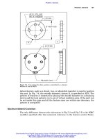
Analysis of a Composite Geometric Tolerance
A pattern of features controlled with composite tolerancing can be inspected
with a set of functional gages. Each segment of the feature control frame rep-
resents a gage. To inspect the pattern of holes in Fig. 13-1, the pattern-locating
control, the upper segment of the feature control frame, consists of three mu-
tually perpendicular planes, datums A, B, and C, and four virtual condition
pins .242 in diameter. The feature-relating control, the lower segment of the
feature control frame, consists of only one plane, datum A, and four virtual
condition pins .250 in diameter. These two gages are required to inspect this
2
2.000
4
Unless Otherwise Specified:
.XXX = ± .005
ANGLES = ± 1°
1.000
B
A
3
4X Ø .252 265

5.000
4.000
1
1.000
2.000
1.000
C
Figure 13-1 A pattern of features controlled with a composite tolerance.
Downloaded from Digital Engineering Library @ McGraw-Hill (www.digitalengineeringlibrary.com)
Copyright © 2006 The McGraw-Hill Companies. All rights reserved.
Any use is subject to the Terms of Use as given at the website.
Graphic Analysis
P1: PBU
MHBD031-13 MHBD031-Cogorno-v6.cls April 11, 2006 17:1
210 Chapter Thirteen
TABLE 13-1 Inspection Data Derived from a Part Made from Specifications in the Drawing
in Fig. 13-1
Feature Feature
location location Feature-to-
from from Departure Datum-to-pattern feature
Feature datum C datum B Feature from MMC tolerance tolerance
number X-axis Y-axis size (bonus) zone size zone size
1 .997 1.003 Ø.256 .004 Ø.014 Ø.006
2 1.004 3.004 Ø.258 .006 Ø.016 Ø.008
3 3.006 2.998 Ø.260 .008 Ø.018 Ø.010
4 3.002 .998 Ø.254 .002 Ø.012 Ø.004
pattern. If gages are not available, graphic analysis can be used. The procedure
for inspecting composite tolerancing with graphic analysis is presented below.
The following is the sequence of steps for generating a data graph for the
graphic analysis of a composite tolerance:

1. Collect the inspection data shown in Table 13-1.
2. On a piece of graph paper, select an appropriate scale, and draw the specified
datums. This sheet is called the data graph. The drawing, the upper segment
of the composite feature control frame, and the inspection data dictate the
configuration of the data graph.
3. From the drawing, determine the true position of each feature, and draw the
centerlines on the data graph.
4. Since tolerances are in the magnitude of thousandths of an inch, a second
scale, called the deviation scale, is established. Typically, one square on the
graph paper equals .001 of an inch on the deviation scale.
5. Draw the appropriate diameter tolerance zone around each true position by
using the deviation scale. For the drawing in Fig. 13-1, each tolerance zone
is a circle with a diameter of .010 plus its bonus tolerance. The datum-to-
pattern tolerance zone diameters are listed in Table 13-1.
6. Draw the actual location of each feature axis on the data graph. If the loca-
tion of any of the feature axes falls outside the feature’s respective circular
tolerance zone, the datum-to-pattern relationship is out of tolerance and the
Figure 13-2 The upper segment of the composite
feature control frame in Fig. 13-1.
Downloaded from Digital Engineering Library @ McGraw-Hill (www.digitalengineeringlibrary.com)
Copyright © 2006 The McGraw-Hill Companies. All rights reserved.
Any use is subject to the Terms of Use as given at the website.
Graphic Analysis
P1: PBU
MHBD031-13 MHBD031-Cogorno-v6.cls April 11, 2006 17:1
Graphic Analysis 211
1.000
1.000
2.000
Datum B

Datum C
2.000
Figure 13-3 The data graph with tolerance zones and feature axes for the data in Table 13-1.
part is rejected. If all of the axes fall inside their respective tolerance zones,
the datum-to-pattern relationship is in tolerance, but the pattern must be
further evaluated to satisfy the feature-to-feature relationships.
The following is the sequence of steps for generating a tolerance zone overlay
gage for the graphic analysis evaluation of a composite tolerance:
1. Place a piece of tracing paper over the data graph. Trace the true posi-
tion axes on the tracing paper. This sheet is called the tolerance zone over-
lay gage. The drawing, the lower segment of the feature control frame, and
Figure 13-4 The lower segment of the composite
feature control frame in Fig. 13-1.
Downloaded from Digital Engineering Library @ McGraw-Hill (www.digitalengineeringlibrary.com)
Copyright © 2006 The McGraw-Hill Companies. All rights reserved.
Any use is subject to the Terms of Use as given at the website.
Graphic Analysis
P1: PBU
MHBD031-13 MHBD031-Cogorno-v6.cls April 11, 2006 17:1
212 Chapter Thirteen
2.000
2.000
Figure 13-5 The tolerance zone overlay gage.
the inspection data dictate the configuration of the tolerance zone overlay
gage.
2. Draw the appropriate feature-to-feature positional tolerance zones around
each true position axis on the tracing paper. Each tolerance zone is a cir-
cle with a diameter of .002 plus its bonus tolerance. The feature-to-feature
tolerance zone diameters are listed in Table 13-1.
3. If the tracing paper can be adjusted to include all actual feature axes within

the tolerance zones on it, the feature-to-feature relationships are in toler-
ance. If each axis simultaneously falls inside both of its respective tolerance
zones, the pattern is acceptable.
When the tolerance zone overlay gage is placed over the data graph in Fig.
13-6, the axes of holes 1 through 3 can easily be placed inside their respective
tolerance zones. The axis of the fourth hole, however, will not fit inside the
fourth tolerance zone. Therefore, the pattern is not acceptable. It is easy to see
on the data graph that this hole can be reworked. Simply enlarging the fourth
hole by about .004 will make the pattern acceptable.
Downloaded from Digital Engineering Library @ McGraw-Hill (www.digitalengineeringlibrary.com)
Copyright © 2006 The McGraw-Hill Companies. All rights reserved.
Any use is subject to the Terms of Use as given at the website.
Graphic Analysis
P1: PBU
MHBD031-13 MHBD031-Cogorno-v6.cls April 11, 2006 17:1
Graphic Analysis 213
1.000
1.000 2.000
Datum B
Datum C
2.000
Figure 13-6 The tolerance zone overlay gage is placed on top of the data graph.
Analysis of a Pattern of Features Controlled to a
Datum Feature of Size
A pattern of features controlled to a datum feature of size specified at MMC is a
very complicated geometry that can easily be inspected with graphic analysis.
The following is the sequence of steps for generating a data graph for the
graphic analysis evaluation of a pattern of features controlled to a datum fea-
ture of size:
1. Collect the inspection data shown in Table 13-2.

2. On the data graph, select an appropriate scale, and draw the specified da-
tums. The drawing, the feature control frame controlling the hole pattern,
and the inspection data dictate the configuration of the data graph.
3. From the drawing, determine the true position of the datum feature and the
true position of each feature in the pattern. Draw their centerlines on the
data graph.
4. Establish a deviation scale. Typically one square on the graph paper equals
.001 of an inch on the deviation scale.
Downloaded from Digital Engineering Library @ McGraw-Hill (www.digitalengineeringlibrary.com)
Copyright © 2006 The McGraw-Hill Companies. All rights reserved.
Any use is subject to the Terms of Use as given at the website.
Graphic Analysis
P1: PBU
MHBD031-13 MHBD031-Cogorno-v6.cls April 11, 2006 17:1
214 Chapter Thirteen
A
4
B
D
Ø .505 520
3
4.000
4.000
4X Ø .255 265
3.000
3.000
1
C
2
Figure 13-7 The drawing of a pattern of features controlled to a datum feature of

size.
5. Draw the appropriate diameter tolerance zone around each true position
using the deviation scale. For the drawing in Fig. 13-7, each tolerance zone
is a circle with a diameter of .005 plus its bonus tolerance. The total geometric
tolerance diameters are listed in Table 13-2.
6. Draw the actual location of each feature on the data graph. If each feature
axis falls inside its respective tolerance zone, the part is in tolerance. If one
or more feature axes fall outside their respective tolerance zones, the part
may still be acceptable if there is enough shift tolerance to shift all the axes
into their respective tolerance zones.
TABLE 13-2 Inspection Data Derived from a Part Made from Specifications in the Drawing
in Fig. 13-7
Feature Feature
location from location from Actual Departure Total
Feature datum D datum D feature from MMC geometric
number X-axis Y-axis size (bonus) tolerance
1 −1.997 −1.498 Ø.258 .003 Ø.008
2 −1.998 1.503 Ø.260 .005 Ø.010
3 2.005 1.504 Ø.260 .005 Ø.010
4 2.006 − 1.503 Ø.256 .001 Ø.006
Datum Ø.510 Shift Tolerance = .010
Downloaded from Digital Engineering Library @ McGraw-Hill (www.digitalengineeringlibrary.com)
Copyright © 2006 The McGraw-Hill Companies. All rights reserved.
Any use is subject to the Terms of Use as given at the website.
Graphic Analysis
P1: PBU
MHBD031-13 MHBD031-Cogorno-v6.cls April 11, 2006 17:1
Graphic Analysis 215
Figure 13-8 The feature control frame controlling
the four-hole pattern in Fig. 13-7.

If any of the feature axes falls outside its respective tolerance zone, further
analysis is required. The following is the sequence of steps for generating an
overlay gage for the graphic analysis evaluation of a pattern of features con-
trolled to a datum feature of size:
1. Place a piece of tracing paper over the data graph. This sheet is called the
overlay gage.
2. Trace the actual location of each feature axis on to the overlay gage.
3. Trace the true position axis of datum feature D on to the overlay gage.
4. Trace datum plane B on to the overlay gage.
3.000
4.000
4.000
Datum B
Datum C
3.000
Figure 13-9 The data graph with feature axes and tolerance zone diameters for the data in
Table 13-2.
Downloaded from Digital Engineering Library @ McGraw-Hill (www.digitalengineeringlibrary.com)
Copyright © 2006 The McGraw-Hill Companies. All rights reserved.
Any use is subject to the Terms of Use as given at the website.
Graphic Analysis
P1: PBU
MHBD031-13 MHBD031-Cogorno-v6.cls April 11, 2006 17:1
216 Chapter Thirteen
Datum B
2
3
4
1
Figure 13-10 The overlay gage includes the actual axis of each feature in the pattern,

the shift tolerance zone, and the clocking datum.
5. Calculate the shift tolerance allowed, and draw the appropriate cylindrical
tolerance zone around datum axis D. The shift tolerance equals the difference
between the actual datum feature size and the size at which the datum
feature applies. The virtual condition rule applies to datum D in Fig. 13-7.
Consequently, datum D is .505 at MMC minus .005 (geometric tolerance)
that equals .500 (virtual condition). According to the inspection data, datum
hole D is produced at a diameter of .510. The shift tolerance equals .510
minus .500 or a diameter of .010.
6. If the tracing paper can be adjusted to include all the feature axes on the
overlay gage within its’ shift tolerance zones on the data graph and datum
axis D contained within its shift tolerance zone while orienting datum B
on the overlay gage parallel to datum B on the data graph, the pattern of
features is in tolerance. The graphic analysis in Fig. 13-11 indicates that the
four-hole pattern of features is acceptable.
Graphic analysis is a powerful graphic tool for analyzing part configuration.
This graphic tool is easy to use, accurate, and repeatable. It should be in every
Downloaded from Digital Engineering Library @ McGraw-Hill (www.digitalengineeringlibrary.com)
Copyright © 2006 The McGraw-Hill Companies. All rights reserved.
Any use is subject to the Terms of Use as given at the website.
Graphic Analysis
P1: PBU
MHBD031-13 MHBD031-Cogorno-v6.cls April 11, 2006 17:1
Graphic Analysis 217
3.000
4.000
4.000
Datum B
Datum C
3.000

Datum B on Gage
2
3
1
4
Figure 13-11 The overlay gage placed on top of the data graph.
inspector’s bag of tricks. Graphic analysis is also a powerful analytical tool
engineers can use to better understand how tolerances on drawings will behave.
Summary

The advantages of graphic analysis:

Provides functional acceptance

Reduces time and cost

Eliminates gage tolerance and wear allowance

Allows functional verification of RFS, LMC, as well as MMC

Allows verification of a tolerance zone of any shape

Provides a visual record for the material review board

Minimizes storage required for gages

The accuracy of graphic analysis:
The accuracy of graphic analysis is affected by such factors as the accu-
racy of the graphs and overlay gage, the accuracy of the inspection data, the
Downloaded from Digital Engineering Library @ McGraw-Hill (www.digitalengineeringlibrary.com)

Copyright © 2006 The McGraw-Hill Companies. All rights reserved.
Any use is subject to the Terms of Use as given at the website.
Graphic Analysis
P1: PBU
MHBD031-13 MHBD031-Cogorno-v6.cls April 11, 2006 17:1
218 Chapter Thirteen
completeness of the inspection process, and the ability of the drawing to pro-
vide common drawing interpretations.

Sequence of steps for the analysis of composite geometric tolerance:
1. Draw the datums, the true positions, the datum-to-pattern tolerance zones,
and the actual feature locations on the data graph.
2. On a piece of tracing paper placed over the data graph, trace the true po-
sitions, and construct the feature-to-feature tolerance zones. This sheet is
called the tolerance zone overlay gage.
3. Adjust the tolerance zone overlay gage to fit over the actual feature locations.
If each actual feature location falls inside both of its respective tolerance
zones, the pattern of features is in tolerance.
Sequence of steps for the analysis of a pattern of features controlled to a datum
feature of size:
1. Draw the datums, the true positions, the tolerance zones, and the ac-
tual feature locations on the data graph. If the actual feature locations
fall inside the tolerance zones, the part is good, and no further analysis
is required. Otherwise, continue to step two to utilize the available shift
tolerance.
2. On a piece of tracing paper placed over the data graph, trace the actual
feature locations, the clocking datum, and the true position of the da-
tum feature of size. Then, draw the shift tolerance zone about the true
position of the datum feature of size. This sheet is called the overlay
gage.

3. Adjust the overlay gage to fit over the actual feature locations while keeping
the shift tolerance zone over the axis on the data gage and the clocking da-
tums aligned. If each actual feature location falls inside both of its respective
tolerance zones, the pattern of features is in tolerance.
Chapter Review
1. List the advantages of graphic analysis.
Downloaded from Digital Engineering Library @ McGraw-Hill (www.digitalengineeringlibrary.com)
Copyright © 2006 The McGraw-Hill Companies. All rights reserved.
Any use is subject to the Terms of Use as given at the website.
Graphic Analysis
P1: PBU
MHBD031-13 MHBD031-Cogorno-v6.cls April 11, 2006 17:1
Graphic Analysis 219
2. List the factors that affect the accuracy of graphic analysis.
Figure 13-12 Refer to the feature control frame for
questions 3 through 7.
3. A piece of graph paper with datums, true positions, tolerance zones, and
actual feature locations drawn on it is called a
.
4. A piece of tracing paper with datums, true positions, tolerance zones, and
actual feature locations traced or drawn is called a
.
5. The upper segment of the composite feature control frame, the drawing, and
the inspection data dictates the configuration of the
.
6. The lower segment of the feature control frame, the drawing, and the inspec-
tion data dictate the configuration of the
.
7. If the tracing paper can be adjusted to include all feature axes within the
on the tracing paper, the feature-to-feature

relationships are in tolerance.
Figure 13-13 Refer to the feature control frame for
questions 8 through 11.
8. To inspect a datum feature of size, the feature control frame, the drawing,
and the inspection data dictate the configuration of the
.
9. Draw the actual location of each feature on the data graph. If each feature
axis falls inside its respective tolerance zone, the part is
.
10. If any of the feature axes falls outside its respective tolerance zone,
.
.
11. If the tracing paper can be adjusted to include all the feature axes within the
tolerance zones on the data graph and the datum axis contained within its
tolerance zone while keeping the pattern parallel to datum B, the pattern
of features is
.
Downloaded from Digital Engineering Library @ McGraw-Hill (www.digitalengineeringlibrary.com)
Copyright © 2006 The McGraw-Hill Companies. All rights reserved.
Any use is subject to the Terms of Use as given at the website.
Graphic Analysis
P1: PBU
MHBD031-13 MHBD031-Cogorno-v6.cls April 11, 2006 17:1
220 Chapter Thirteen
2.000
2
A
B
1.000
Unless Otherwise Specified:

.XXX = ± .005
ANGLES = ± 1°
4
3
4X Ø .190 205
5.000
4.000
C
1.000
2.000
1.000
1
Figure 13-14
A pattern of features controlled with a composite tolerance: Problem 1.
TABLE
13-3 Inspection Data for Graphic Analysis of Problem 1
Feature Feature
location location Datum-to- Feature-to-
from from Departure pattern feature
Feature datum C datum B Feature from MMC tolerance tolerance
number X-axis Y-axis size (bonus) zone size zone size
1 1.002 1.003 Ø.200
2 1.005 3.006 Ø.198
3 3.005 3.002 Ø.198
4 3.003 .998 Ø.196
Problems
1. A part was made from the drawing in Fig. 13-14; the inspection data was
tabulated in Table 13-3. Perform a graphic analysis of the part. Is the pattern
within tolerance?
If it is not in tolerance, can it be reworked? If so, how?

Downloaded from Digital Engineering Library @ McGraw-Hill (www.digitalengineeringlibrary.com)
Copyright © 2006 The McGraw-Hill Companies. All rights reserved.
Any use is subject to the Terms of Use as given at the website.
Graphic Analysis
P1: PBU
MHBD031-13 MHBD031-Cogorno-v6.cls April 11, 2006 17:1
Graphic Analysis 221
2
2.000
4
Unless Otherwise Specified:
.XXX = ± .005
ANGLES = ± 1°
1.000
B
A
3
4X Ø .166 180
5.000
4.000
1
1.000
2.0001.000
C
Figure 13-15 A pattern of features controlled with a composite tolerance: Problem 2.
TABLE 13-4 Inspection Data for Graphic Analysis of Problem 2
Feature Feature
location location Datum-to- Feature-to-
from from Departure pattern feature
Feature datum C datum B Feature from MMC tolerance tolerance

number X-axis Y-axis size (bonus) zone size zone size
1 1.004 .998 Ø.174
2 .995 3.004 Ø.174
3 3.000 3.006 Ø.172
4 3.006 1.002 Ø.176
2. A part was made from the drawing in Fig. 13-15; the inspection data was
tabulated in Table 13-4. Perform a graphic analysis of the part. Is the pattern
within tolerance?
If it is not in tolerance, can it be reworked? If so, how?
Downloaded from Digital Engineering Library @ McGraw-Hill (www.digitalengineeringlibrary.com)
Copyright © 2006 The McGraw-Hill Companies. All rights reserved.
Any use is subject to the Terms of Use as given at the website.
Graphic Analysis
P1: PBU
MHBD031-13 MHBD031-Cogorno-v6.cls April 11, 2006 17:1
222 Chapter Thirteen
A
4
B
D
Ø .505 530
3
4X Ø .270 285
4.000
4.000
3.000
3.000
1
C
2

Figure 13-16
A pattern of features controlled to a size feature: Problem 3.
TABLE 13-5 Inspection Data for Graphic Analysis of Problem 3
Feature Feature
location from location from Actual Departure Total
Feature datum D datum D feature from MMC geometric
number X-axis Y-axis size (bonus) tolerance
1 −1.992 −1.493 Ø.278
2 −1.993 1.509 Ø.280
3 2.010 1.504 Ø.280
4 2.010 −1.490 Ø.282
Datum Ø.520
Shift Tolerance =
3. A part was made from the drawing in Fig. 13-16; the inspection data was
tabulated in Table 13-5. Perform a graphic analysis of the part. Is the pattern
within tolerance?
If it is not in tolerance, can it be reworked? If so, how?
Downloaded from Digital Engineering Library @ McGraw-Hill (www.digitalengineeringlibrary.com)
Copyright © 2006 The McGraw-Hill Companies. All rights reserved.
Any use is subject to the Terms of Use as given at the website.
Graphic Analysis
P1: PBU
MHBD031-13 MHBD031-Cogorno-v6.cls April 11, 2006 17:1
Graphic Analysis 223
A
4
B
Ø .375 390
D
3

4X Ø .214 225
4.000
4.000
3.000
3.000
1
C
2
Figure 13-17
A pattern of features controlled to a size feature: Problem 4.
TABLE
13-6 Inspection Data for Graphic Analysis of Problem 4
Feature Feature
location from location from Actual Departure Total
Feature datum D datum D feature from MMC geometric
number X-axis Y-axis size (bonus) tolerance
1 −1.995 −1.495 Ø.224
2 −1.996 1.503 Ø.218
3 2.005 1.497 Ø.220
4 1.997 −1.506 Ø.222
Datum Ø.380
Shift Tolerance =
4. A part was made from the drawing in Fig. 13-17; the inspection data was
tabulated in Table 13-6.
Perform a graphic analysis of the part. Is the pattern within tolerance?
If it is not in tolerance, can it be reworked? If so, how?
Downloaded from Digital Engineering Library @ McGraw-Hill (www.digitalengineeringlibrary.com)
Copyright © 2006 The McGraw-Hill Companies. All rights reserved.
Any use is subject to the Terms of Use as given at the website.
Graphic Analysis

P1: PBU
MHBD031-13 MHBD031-Cogorno-v6.cls April 11, 2006 17:1
224
Downloaded from Digital Engineering Library @ McGraw-Hill (www.digitalengineeringlibrary.com)
Copyright © 2006 The McGraw-Hill Companies. All rights reserved.
Any use is subject to the Terms of Use as given at the website.
Graphic Analysis
P1: PBU
MHBD031-14 MHBD031-Cogorno-v6.cls April 11, 2006 21:50
Chapter
14
A Strategy for Tolerancing Parts
When tolerancing a part, the designer must determine the attributes of each
feature or pattern of features and the relationships of these features with one
another. In other words, what are the size, the size tolerance, the location di-
mensions, and the location and orientation tolerances of each feature? At what
material conditions do these size features apply? Which are the most appro-
priate datum features? All of these questions must be answered in order to
properly tolerance a part. Some designers believe that parts designed with a
solid modeling CAD program do not require tolerancing. A note in the Dimen-
sioning and Tolerancing standard indicates caution when designing parts with
solid modeling. The standard reads: “CAUTION: If CAD/CAM database models
are used and they do not include tolerances, then tolerances must be expressed
outside of the database to reflect design requirements.” One way or another,
each feature must be toleranced.
Chapter Objectives
After completing this chapter, you will be able to

Tolerance size features located to plane surface features


Tolerance size features located to size features

Tolerance a pattern of features located to a second pattern of features
Size Features Located to Plane Surface Features
The first step in tolerancing a size feature, such as the hole in Fig. 14-1, is to
specify the size and size tolerance of the feature. The size and the size tolerance
may be determined by using one of the fastener formulas, a standard fit table,
or the manufacturer’s specifications. The second step is locating and orient-
ing the size feature. The location tolerance comes from the size tolerance. If a
225
Downloaded from Digital Engineering Library @ McGraw-Hill (www.digitalengineeringlibrary.com)
Copyright © 2006 The McGraw-Hill Companies. All rights reserved.
Any use is subject to the Terms of Use as given at the website.
Source: Geometric Dimensioning and Tolerancing for Mechanical Design
P1: PBU
MHBD031-14 MHBD031-Cogorno-v6.cls April 11, 2006 21:50
226 Chapter Fourteen
Ø 2.010- 2.030
4.00
3.000
2.000
6.00
2.00
Figure 14-1
A size feature located to plane surfaces on an untoleranced drawing.
Ø 2.000-inch mating feature must fit through the hole in Fig. 14-4, the loca-
tion tolerance can be as large as the difference between the Ø 2.010 hole and
the Ø 2.000-inch mating feature or a positional tolerance of Ø .010. A posi-
tional tolerance for locating and orienting a feature of size is always specified
with a material condition modifier. The maximum material condition modifier

(circle M) has been specified for the hole in Fig. 14-4. The MMC modifier is typ-
ically specified for features in static assemblies. The RFS modifier is typically
used for high-speed, dynamic assemblies. The LMC modifier is used where a
specific minimum edge distance must be maintained. The size tolerance not
only controls the feature’s size but also controls the feature’s form (Rule #1).
According to the drawing in Fig. 14-1, the size tolerance for the Ø 2.000-inch
hole can be as large as .020. The machinist can make the hole diameter any-
where between 2.010 and 2.030. However, if the machinist actually produces
the hole at Ø 2.020, according to Rule #1, the form tolerance for the hole is
.010, that is, 2.020 minus 2.010. The hole must be straight and round within
.010. The hole size can be produced even larger, up to Ø 2.030, in which case
the form tolerance is even larger. If the straightness or circularity tolerance,
automatically implied by Rule #1, does not satisfy the design requirements, an
appropriate form tolerance must be specified.
The next step in tolerancing a size feature is to identify the location datums.
The hole in Fig. 14-1 is dimensioned up from the bottom edge and over from the
left edge. Consequently, the bottom and left edges are implied location datums.
When geometric dimensioning and tolerancing is applied, these datums must be
specified. If the designer has decided that the bottom edge is more important to
the part design than the left edge, the datum letter for the bottom edge, datum
B, will precede the datum letter for the left edge, datum C, in the feature control
frame.
Downloaded from Digital Engineering Library @ McGraw-Hill (www.digitalengineeringlibrary.com)
Copyright © 2006 The McGraw-Hill Companies. All rights reserved.
Any use is subject to the Terms of Use as given at the website.
A Strategy for Tolerancing Parts