FUNDAMENTALS OF CONTACT BETWEEN SOLIDS 475
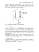
Radius r
Angular
velocity ω
Elastic
deformation
of contact
∆r
Tangential velocity, v
1

= ωr
Tangential
velocity, v
1

= ωr
Tangential
velocity
v
2
= ω(r − ∆r)
Micro-slip compensates
for lower surface speed,


v
1

- v
2

= ω∆r
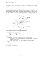
FIGURE 10.23 Schematic illustration of micro-slip and creeping movement in a rolling
contact.
When the roller or sphere sustains traction, the micro-slip increases in level and extent over
the rolling contact area [94,95]. When micro-slip prevails over the entire rolling contact area,
gross sliding or skidding of the roller (or sphere) will commence.
A fundamental difference between rolling and sliding friction is that other energy dissipation
mechanisms, which are negligible for sliding friction, become significant for rolling because
of the very low friction level. Major sources of energy dissipation, which are not discussed
further here, are aerodynamic drag of the rapidly rotating roller and repetitive compression
of air inside a pneumatic tyre. Another important source of energy dissipation is hysteresis in
the mechanical response of the rolling material. Hysteresis means that the compressive
stresses ahead of the centre of the rolling contact are greater than the compressive stresses
behind the rolling contact. Ahead is defined as not yet reached by the centre of the rolling
contact while behind is defined as already rolled on by the centre of the rolling contact. The
resulting asymmetry in compressive stresses generates reaction forces that oppose the rolling
motion. For example, hysteresis is found to be the principal component of rolling friction in
polymers [87]. An effect similar to mechanical hysteresis may also be generated by adhesion
between the roller and rolled surface [96]. Adhesion behind the rolling contact causes the
compressive forces behind the rolling contact to be less than the compressive forces ahead of
the rolling contact. Adhesive effects are significant for rubbers [96] where the adhesion is
generated by van der Waals bonding between atoms of the opposing surfaces [97].
Rolling is nearly always associated with high levels of contact stress, which can be sufficient
at high contact loads to cause plastic deformation in the rolling contact. Plastic deformation
not only causes the surface layers of the roller and rolled surface to accumulate plastic strain,
but may also cause corrugation to occur. Corrugation is the transformation of a smooth, flat
surface into a surface covered by a wave-form like profile aligned so that the troughs and
valleys of the wave-form profile lie perpendicular to the direction of rolling. The wavelength
of corrugations varies from 0.3 [mm] on the discs of Amsler test machines to 40 ~ 80 [mm] on
railway tracks [98]. Another term used to describe corrugations, especially longer wavelength

corrugations, is facets. Although the causes of corrugation are unclear, there is evidence that
vibration of the rolling wheel and metallurgical factors exhibit a strong influence [99,100]. It
was found that the peaks of the corrugations on steel surfaces were significantly harder than
the troughs between the corrugations [101]. It is believed that corrugation occurs when a
lump of plastically deformed material is formed at the leading edge of the rolling contact.
TEAM LRN
476 ENGINEERING TRIBOLOGY
This lump periodically grows to a maximum size before being released behind the rolling
contact to form a corrugation [88,89].
According to theoretical models of the deformation and slip involved in rolling friction, it
appears that there is a linear relationship between contact force and the drag force opposing
rolling [84]. The geometry of the rolling contact has a strong influence on rolling friction, and
the coefficient of rolling friction is inversely related to the rolling radius. At low loads where
elastic deformation dominates, the coefficient of rolling friction is inversely proportional to
the square root of the rolling radius, at higher contact loads where plastic deformation is
significant, the coefficient of rolling friction is inversely proportional to the rolling radius
[90]. Basic materials parameters also exert an effect, the coefficient of rolling friction is
inversely related to the Young's modulus of the rolling material [90]. Temperature exerts a
strong effect on the coefficient of rolling friction of polymers since the mechanical hysteresis
of the polymer is controlled by temperature [92]. The coefficient of adhesion in a rolling steel
contact was found to decline with speed in the range of 20 [km/hr] to 500 [km/hr] [91].
Concentration of Frictional Heat at the Asperity Contacts
The inevitable result of friction is the release of heat and, especially at high sliding speeds, a
considerable amount of energy is dissipated in this manner. The released heat can have a
controlling influence on friction and wear levels due to its effect on the lubrication and wear
processes. Almost all of the frictional heat generated during dry contact between bodies is
conducted away through the asperities in contact [24]. Since the true contact area between
opposing asperities is always considerably smaller than the apparent contact area, the
frictional energy and resulting heat at these contacts becomes highly concentrated with a
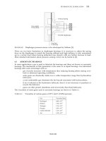
correspondingly large temperature rise as illustrated schematically in Figure 10.24.

Load
Frictional
temperature
rise if energy
is dissipated
uniformly
Actual
temperature
rise
Sliding speed
Frictional
power
Frictional power to sustain sliding is dissipated as heat over small asperity contact areas
FIGURE 10.24 Concentration of frictional energy at the asperity contacts.
This concentration of frictional energy over small localized areas has a significant influence
on friction and wear. Local temperatures can rise to very high values even with a relatively
small input of frictional energy. For example, a frictional temperature rise was exploited by
paleolithic man to ignite fires by rotating a stick against a piece of wood.
TEAM LRN
FUNDAMENTALS OF CONTACT BETWEEN SOLIDS 477
Surface heating from frictional energy dissipation also causes the surface layers of a material
to expand. Where such heating is localized, a small area of surface becomes elevated from the
rest of the surface which has not sustained thermal expansion. This effect is known as a
‘thermal mound’ since the shape of this temperature-induced structure resembles a gently
sloping hill or mound. When the wearing surface is flat, the distribution of thermal mounds
tend to be random along with the distribution of frictional energy dissipation. When the
contact of the wearing surface is controlled by asperities, the asperities which sustain the
greatest amount of frictional energy dissipation will expand the most and lift apart the
remaining asperities. The effect of thermal mound formation results in the concentration of
frictional energy dissipation and mechanical load on a few asperities only. This effect is

transient and once the source of frictional energy is removed, i.e. by stopping the moving
surfaces, the thermal mounds disappear.
Shear rates between contacting solids can also be extremely high as often only a thin layer of
material accommodates the sliding velocity difference. The determination of surface
temperature as well as the observation of wear is difficult as the processes are hindered by the
contacting surfaces. In the majority of sliding contacts, the extremes of temperature, stress
and strain can only be assessed indirectly by their effect on wear particles and worn surfaces.
The frictional temperatures can, for example, be measured by employing the ‘dynamic
thermocouple method’ [24]. The method involves letting two dissimilar metals slide against
each other. Frictional temperature rises at the sliding interface cause a thermo-electric
potential to develop which can be measured. For example, significant temperature rises were
detected by this method when constantan alloy was slid under unlubricated conditions
against steel at a velocity of 3 [m/s] [24]. Momentary temperature rises reaching 800°C but
only lasting for approximately 0.1 [ms] occurring on a random basis were observed. It is
speculated that these temperature rises are the result of intense localized metal deformation
between asperities in contact.
Wear Between Surfaces of Solids
As already discussed the contact between surfaces of solids at moderate pressures is limited to
contacts between asperities of opposing surfaces. Most forms of wear are the result of events
occurring at asperity contacts. There could, however, be some exceptions to this rule, e.g.
erosive wear which involves hard particles colliding with a surface.
It has been postulated by Archard that the total wear volume is proportional to the real
contact area times the sliding distance [37]. A coefficient ‘K’ which is the proportionality
constant between real contact area, sliding distance and the wear volume has been
introduced, i.e.:
V = K A
r
l = K l
H
W

(10.9)
where:
V is the wear volume [m
3
];
K is the proportionality constant;
A
r
is the real area of the contact [m
2
];
W is the load [N];
H is the hardness of the softer surface [Pa];
l is the sliding distance [m].
TEAM LRN
478 ENGINEERING TRIBOLOGY
The ‘K’ coefficient, also known as the ‘Archard coefficient’ is widely used as an index of wear
severity. The coefficient can also be imagined as the proportion of asperity contacts resulting
in wear. The value of ‘K’ is never supposed to exceed unity and in practice ‘K’ has a value of
0.001 or less for all but the most severe forms of wear. The low value of ‘K’ indicates that
wear is caused by only a very small proportion of asperity contacts. In almost all cases,
asperities slide over each other with little difficulty and only a minute proportion of asperity
contacts result in the formation of wear particles.
It has also been suggested that wear particles are the result of a cumulative process of many
interactions between randomly selected opposing asperities [38]. The combination of
opposing asperities during sliding at any one moment can easily be imagined as
continuously changing. A gradual or incremental mode of wear particle formation allows for
extensive freedom for variation or instability in the process. Statistical analysis of wear data
reveals that there is a short term ‘memory’ inherent in wear processes, i.e. any sample of a
wear rate is related to the immediately preceding wear rates, although there seems to be no

correlation with much earlier wear rates [39]. Therefore wear prediction is extremely difficult.
10.5 SUMMARY
Real surfaces are composed of surface features ranging in size from individual atoms to
visible grooves and ridges. Most surface features affect wear and friction. Since almost all
surfaces are rough, in terms of solid contact they cannot be approximated by a flat plane. The
basic laws of friction are a result of the control of solid contact by rough surfaces. The
topography of the contacting surfaces therefore has a decisive effect on wear and friction.
Rough surfaces have very small areas of real contact with the opposing surface and this
causes wear and friction to be determined by high contact stresses and extreme concentrations
of frictional energy even though the nominal contact stress and total frictional energy can be
small.
Friction has traditionally been divided into static and kinetic friction. Exact measurements of
microscopic sliding movements reveal that as the friction force acting on a contact is
progressively increased, microscopic sliding movement occurs for all levels of friction force
and the maximum friction force occurs at some specific sliding speed. The basic difference
between gross sliding and sliding movements at small levels of friction force is that these
latter movements are reversible. A major consequence of the difference between static and
kinetic coefficients of friction is ‘stick-slip’ or discontinuous sliding. Stick-slip is often present
when the supporting structure of the sliding contact has insufficient stiffness to follow the
rapid changes in frictional force that can occur.
Wear results from direct contact between the individual asperities at sliding interfaces and,
in almost all situations, many asperity interactions are required before wear occurs.
REFERENCES
1 J. Benard (editor), Adsorption on Metal Surfaces, Elsevier, Amsterdam, 1983.
2 D. Landheer, A.J.G. Dackus and J.A. Klostermann, Fundamental Aspects and Technological Implications of
the Solubility Concept for the Prediction of Running Properties, Wear, Vol. 62, 1980, pp. 255-286.
3 E.A. Gulbransen, The Role of Minor Elements in the Oxidation of Metals, Corrosion, Vol. 12, 1956, pp. 61-67.
4 K. Meyer, Physikalisch-Chemische Kristallographie, Copyright VEB Deutscher Verlag fur
Grundstoffindustrie, Leipzig, Gutenberg Buchdruckerei, Weimar, 1988.
5 D.H. Buckley, Surface Effects in Adhesion, Friction, Wear and Lubrication, Elsevier, Amsterdam, 1981.

6 D. Godfrey, Chemical Changes in Steel Surfaces During Extreme-Pressure Lubrication, ASLE Transactions,
Vol. 5, 1962, pp. 51-66.
7 R. Kothari and R.W. Vook, The Effect of Cold Work on Surface Segregation of Sulphur on Oxygen-Free High
Conductivity Copper, Wear, Vol. 157, 1992, pp. 65-79.
TEAM LRN
FUNDAMENTALS OF CONTACT BETWEEN SOLIDS 479
8 J. Van Alsten and S. Granick, Friction Measured With a Surface Forces Apparatus, Tribology Transactions,
Vol. 32, 1989, pp. 246-250.
9 T.R. Thomas (editor), Rough Surfaces, Longman Group Limited, 1982.
10 A. Majumdar and B. Bhushan, Fractal Model of Elastic-Plastic Contact Between Rough Surfaces, Transactions
ASME, Journal of Tribology, Vol. 113, 1991, pp. 1-11.
11 E.J. Abbott and F.A. Firestone, Specifying Surface Quality, Mechanical Engineering, Vol. 55, 1933, pp. 569-
572.
12 E.F. Finklin, The Bearing Area of Surfaces, Transactions ASME, Journal of Lubrication Technology, Vol. 90,
1968, pp. 329-330.
13 R.S. Sayles and T.R. Thomas, A Stochastic Explanation of Some Structural Properties of a Ground Surface, Int.
Journal of Production Research, Vol. 14, 1976, pp. 641-655.
14 J.A. Greenwood and J.B.P. Williamson, Contact of Nominally Flat Surfaces, Proc. Roy. Soc., London, Series A,
Vol. 295, 1966, pp. 300-319.
15 J.B.P. Williamson, The Microtopography of Surfaces, Proc. Inst. of Mech. Engrs., Vol. 182, Pt. 3K, 1967-1968,
pp. 21-30.
16 R.S. Sayles and T.R. Thomas, The Spatial Representation of Surface Roughness by Means of the Structure
Function: a Practical Alternative to Correlation, Wear, Vol. 42, 1977, pp. 263-276.
17 R.S. Sayles and T.R. Thomas, Surface Topography as a Non-Stationary Random Process, Nature, Vol. 271,
1978, pp. 431-434.
18 J.I. McCool, Relating Profile Instrument Measurements to the Functional Performances of Rough Surfaces,
Transactions ASME, Journal of Tribology, Vol. 109, 1987, pp. 264-270.
19 A. Majumdar and B. Bhushan, Role of Fractal Geometry in Roughness Characterization and Contact
Mechanics of Surfaces, Transactions ASME, Journal of Tribology, Vol. 112, 1990, pp. 205-216.
20 A. Majumdar and C.L. Tien, Fractal Characterization and Simulation of Rough Surfaces, Wear, Vol. 136,

1990, pp. 313-327.
21 M.V. Berry and Z.V. Lewis, On the Weierstrass-Mandelbrot Fractal Function, Proc. Roy. Soc., London, Series
A, Vol. 370, 1980, pp. 459-484.
22 W. Hirst and A.E. Hollander, Surface Finish and Damage in Sliding, Proc. Roy. Soc., London, Series A, Vol.
337, 1974, pp. 379-394.
23 H. Czichos, Tribology; A System Approach to the Science and Technology of Friction, Lubrication and Wear,
Elsevier, Amsterdam, 1978.
24 F.P. Bowden and D. Tabor, The Friction and Lubrication of Solids, Part I, Clarendon Press, Oxford, 1954.
25 D.J. Whitehouse and J.F. Archard, The Properties of Random Surfaces of Significance in Their Contact, Proc.
Roy. Soc. London, Series A, Vol. 316, 1970, pp. 97-121.
26 R.A. Onions and J.F. Archard, The Contact of Surfaces Having a Random Structure, Journal of Physics, Series
D: Appl. Phys., Vol. 6, 1973, pp. 289-304.
27 J.F. Archard, Elastic Deformation and the Laws of Friction, Proc. Roy. Soc., London, Series A, Vol. 243, 1957,
pp. 190-205.
28 J. Pullen and J.B.P. Williamson, On the Plastic Contact of Rough Surfaces, Proc. Roy. Soc., London, Series A,
Vol. 327, 1972, pp. 159-173.
29 P.R. Nayak, Random Process Model of Rough Surfaces, Transactions ASME, Journal of Lubrication Technology,
Vol. 93, 1971, pp. 398-407.
30 A.W. Bush, R.D. Gibson and T. R Thomas, The Elastic Contact of a Rough Surface, Wear, Vol. 35, 1975, pp. 87-
111.
31 P.K. Gupta and N.H. Cook, Junction Deformation Models for Asperities in Sliding Interactions, Wear, Vol. 20,
1972, pp. 73-87.
32 B. Bhushan, Tribology of Mechanics of Magnetic Storage Devices, Sprigler-Verlag, 1990.
33 B. Bhushan, Analysis of the Real Area of Contact Between a Polymeric Magnetic Medium and a Rigid
Surface, Transactions ASME, Journal of Tribology, Vol. 106, 1984, pp. 26-34.
34 J.M. Challen, L.J. MacLean and P.L.B. Oxley, Plastic Deformation of a Metal Surface in Sliding Contact With
a Hard Wedge: Its Relation to Friction and Wear, Proc. Roy. Soc., London, Series A, Vol. 394, 1984, pp. 161-
181.
TEAM LRN
480 ENGINEERING TRIBOLOGY

35 J.T. Burwell and E. Rabinowicz, The Nature of the Coefficient of Friction, Journal of Applied Physics, Vol. 24,
1953, pp. 136-139.
36 M. Eguchi and T. Yamamoto, Dynamic Behaviour of a Slider Under Various Tangential Loading Conditions,
Proc. JSLE. Int. Tribology Conference, 8-10 July 1985, Tokyo, Japan, Elsevier, 1986, pp. 1047-1052.
37 J.F. Archard, Single Contacts and Multiple Encounters, Journal of Applied Physics, Vol. 32, 1961, pp. 1420-
1425.
38 Y. Kimura and H. Okabe, Review of Tribology, Youkandou Press, Tokyo, (in Japanese), 1982.
39 S.C. Lim, C.J. Goh and L.C. Tang, The Interdependence of Wear Events During Slow Sliding - a Statistical
Viewpoint, Wear, Vol. 137, 1990, pp. 99-105.
40 K. Naoi, K. Sasjima and T. Tsukuda, A Quantitative Evaluation of Truncation Wear Based on Three-
Dimensional Surface Asperity Changes, Proc. JAST, Vol. 4, 1999, pp. 452-459.
41 D.J. Whitehouse, Handbook of Surface Metrology, Bristol; Philadelphia: Institute of Physics Pub., 1994.
42 C.Y. Poon, B. Bhushan, Comparison of Surface Roughness Measurements by Stylus Profiler, AFM and Non-
Contact Optical Profiler, Wear, Vol. 190, 1995, pp. 76-88.
43 H. Zahouani, R. Vargiolu, Ph. Kapsa, J.L. Loubat, T.G. Mathia, Effect of Lateral Resolution on
Topographical Images and Three-Dimensional Functional Parameters, Wear, Vol. 219, 1998, pp. 114-123.
44 P. Podsiadlo and G.W. Stachowiak, Scale-Invariant Analysis Tribological Surfaces, Proceedings of the
International Leeds-Lyon Tribology Symposium, ‘Lubrication at the Frontier’, September 1999, Elsevier, 2000.
45 G.W. Stachowiak and P. Podsiadlo, Surface Characterization of Wear Particles, Wear, Vol. 225-229, 1999,
pp. 1171-1185.
46 P. Podsiadlo and G.W. Stachowiak, 3-D Imaging of Wear Particles Found in Synovial Joints, Wear, Vol. 230,
1999, pp. 184-193.
47 W.P. Dong, P.J. Sullivan and K.J. Stout, Comprehensive Study of Parameters for Characterising Three-
Dimensional Topography. IV: Parameters for Characterising Spatial and Hybrid Properties, Wear, Vol. 178,
1994, pp. 45-60.
48 Z. Peng and T.B. Kirk, Two-Dimensional Fast Fourier Transform and Power Spectrum for Wear Particle
Analysis, Tribology International, Vol. 30, 1997, pp. 583-590.
49 D.M. Tsai and C.F. Tseng, Surface Roughness Classification for Castings, Pattern Recognition, Vol. 32, 1999,
pp. 389-405.
50 Y. Wang, K. S. Moon, A methodology for the multi-resolution simulation of grinding wheel surface, Wear,

Vol. 211, 1997, pp. 218-225.
51 X.Q. Jiang, L. Blunt, K.J. Stout, Three-Dimensional Surface Characterization for Orthopaedic Joint
Prostheses, Proceedings of Institute of Mechanical Engineers, Part H, Vol. 213, 1999, pp. 49-68.
52 J L. Starck, F. Murtagh, A. Bijaoui, Image Processing and Data Analysis: The Multiscale Approach, New
York, Cambridge University Press, 1998.
53 G. Borgerfors, Distance Transforms in Arbitrary Dimensions, Comp. Vision, Graphics Image Proc., Vol. 27,
1984, pp. 321-345.
54 P. Grassberger and I. Procaccia, Characterisation of Strange Attractors, Phys. Rev. Letters, Vol. 50, 1983, pp.
346-349.
55 K. Judd, An Improved Estimator of Dimension and Comments on Providing Confidence Intervals, Phys. D.,
Vol. 56, 1992, pp. 216-228.
56 J.C. Russ, Fractal Surfaces, Plenum Press, New York, 1994.
57 M.G. Hamblin and G.W. Stachowiak, Application of the Richardson Technique to the Analysis of Surface
Profiles and Particle Boundaries, Tribology Letters, Vol. 1, 1995, pp. 95-108.
58 W. P. Dong, P. J. Sullivan and K. J. Stout, Comprehensive Study of Parameters for Characterising Three-
Dimensional Surface Topography, II: Statistical Properties of Parameter Variation, Wear, Vol. 167, 1993,
pp. 9-21.
59 M.G. Hamblin and G.W. Stachowiak, Measurement of Fractal Surface Profiles Obtained from Scanning
Electron and Laser Scanning Microscope Images and Contact Profile Meter, Journal of Computer Assisted
Microscopy, Vol. 6, No. 4, 1994, pp. 181-194.
60 C. Tricot, P. Ferland and G. Baran, Fractal Analysis of Worn Surfaces, Wear, Vol. 172, 1994, pp. 127-133.
TEAM LRN
FUNDAMENTALS OF CONTACT BETWEEN SOLIDS 481
61 M. Hasegawa, J. Liu, K. Okuda, M. Nunobiki, Calculation of the Fractal Dimensions of Machined Surface
Profiles, Wear, Vol. 192, 1996, pp. 40-45.
62 J. Lopez, G. Hansali, H. Zahouani, J.C. Le Bosse, T. Mathia, 3D Fractal-Based Characterisation for
Engineered Surface Topography, International Journal of Machine Tools and Manufacture, Vol. 35, 1995, pp.
211-217.
63 S. Ganti, B. Bhushan, Generalized Fractal Analysis and Its Applications to Engineering Surfaces, Wear, Vol.
180, 1995, pp. 17-34.

64 S. Peleg, J. Naor, R. Harley and D. Avnir, Multiresolution texture analysis and classification, IEEE
Transactions on Pattern Analysis Machine Intelligence, Vol. 4 , 1984, pp. 518-523.
65 J.J. Gangepain and C. Roques-Carmes, Fractal Approach to Two Dimensional and Three Dimensional Surface
Roughness, Wear, Vol. 109, 1986, pp. 119-126.
66 K.C. Clarke, Computation of the Fractal Dimension of Topographic Surfaces Using the Triangular Prism
Surface Area Method, Computers and Geosciences, Vol. 12, 1986, pp. 713-722.
67 B. Dubuc, S.W. Zucker, C. Tricot, J-F. Quiniou and D. Wehbi, Evaluating the Fractal Dimension of Surfaces,
Proc. Roy. Soc. London, Series A425, 1989, pp. 113-127.
68 C.A. Brown, P.D. Charles, W.A. Johnsen and S. Chesters, Fractal Analysis of Topographic Data by The
Patchwork Method, Wear, Vol. 161, 1993, pp. 61-67.
69 P. Podsiadlo and G.W. Stachowiak, The Development of Modified Hurst Orientation Transform for the
Characterization of Surface Topography of Wear Particles, Tribology Letters, Vol. 4, 1998, pp. 215-229.
70 P. Prusinkiewicz and A. Lindenmayer, The Algorithmic Beauty of Plants, Springer-Verlag, New York, 1990.
71 M.F. Barsney and L.P. Hurd, Fractals Everywhere, Academic Press, San Diego, 1988.
72 Y. Fisher (editor) Fractal Image Compression. Theory and Application, Springer-Verlag, New York, 1995.
73 K.L. Johnson, Contact Mechanics and the Wear of Metals, Wear, Vol. 190, 1995, pp. 162-170.
74 A. Kapoor, K.L. Johnson and J.A. Williams, A Model for the Mild Ratchetting Wear of Metals, Wear, Vol.
200, 1996, pp. 38-44.
75 A. Kapoor, J.A. Williams and K.L. Johnson, The Steady State Sliding of Rough Surfaces, Wear, Vol. 175,
1995, pp. 81-92.
76 A.F. Bower and K.L. Johnson, The Influence of Strain Hardening on Cumulative Plastic Deformation in
Rolling and Sliding Line Contact, Journal of Mech. Phys. Solids, Vol. 37, 1989, pp. 471-493.
77 B. Bhushan, Contact Mechanics of Rough Surfaces in Tribology: Single Asperity Contact, Appl. Mech. Rev.,
Vol. 49, 1996, pp. 275-298.
78 G. Liu, Q. Wang and C. Lin, A Survey of Current Models for Simulating the Contact Between Rough Surfaces,
Tribology Transactions, Vol. 42, 1999, pp. 581-591.
79 M. Chandrasekaran, A.W. Batchelor and N.L. Loh, Direct Observation of Frictional Seizure of Mild Steel
Sliding on Aluminium by X-ray Imaging, Part 1, Methods, Journal of Materials Science, Vol. 35, 2000, pp.
1589-1596.
80 M. Chandrasekaran, A.W. Batchelor and N.L. Loh, Direct Observation of Frictional Seizure of Mild Steel

Sliding on Aluminium by X-ray Imaging, Part 2, Mechanisms, Journal of Materials Science, Vol. 35, 2000, pp.
1597-1602.
81 A.A. Seireg, Friction and Lubrication in Mechanical Design, Marcel Dekker Inc., New York, 1998.
82 Y. Fu, A.W. Batchelor and N.L. Loh, Study on Fretting Wear Behavior of Laser Treated Coatings by X-ray
Imaging, Wear, Vol. 218, 1998, pp. 250-260.
83 D. Dowson, History of Tribology, Longmans Group, 1979, page 25.
84 J.J. Kalker, Three-Dimensional Elastic Bodies in Rolling Contact, Kluwer Academic Publishers, Dordrecht,
1990.
85 J.J. Kalker, A Fast Algorithm for the Simplified Theory of Rolling Contact, Vehicle System Dynamics, Vol.
11, 1982, pp. 1-13.
86 J.J. Kalker, The Computation of Three-Dimensional Rolling Contact With Dry Friction, Int. Journal for
Numerical Methods in Engineering, Vol. 14, 1979, pp. 1293-1307.
87 D. Tabor, The Mechanism of Rolling Friction; II The Elastic Range, Proc. Roy. Soc., London, Series A, Vol. 229,
1955, pp. 198-220.
TEAM LRN
482 ENGINEERING TRIBOLOGY
88 W.R. Tyfour, J.H. Breynon and A. Kapoor, The Steady State Behaviour of Pearlitic Rail Steel Under Dry
Rolling Sliding Contact Conditions, Wear, Vol. 180, 1995, pp. 79-89.
89 A. Kapoor, Wear by Plastic Ratchetting, Wear, Vol. 212, 1997, pp. 119-130.
90 Y. Uchiyama, Control of Rolling Friction, The Tribologist, Journal of Japanese Society of Tribologists, Vol. 44,
1999, pp. 487-492.
91 K. Ohno, Rolling Friction And Control Between Wheel and Rail, The Tribologist, Journal of Japanese Society
of Tribologists, Vol. 44, 1999, pp. 506-511.
92 I. Sekiguchi, Rolling Friction and Control of Polymeric Materials, The Tribologist, Journal of Japanese Society
of Tribologists, Vol. 44, 1999, pp. 493-499.
93 F.W. Carter, On the Action of a Locomotive Driving Wheel, Proc. Roy. Soc., London, Series A, Vol. 112, 1926,
pp. 151-157.
94 J.J. Kalker, Wheel Rail Rolling Contact Theory, Wear, Vol. 144, 1991, pp. 243-261.
95 K.L. Johnson, Contact Mechanics, Cambridge University Press, Cambridge, 1985.
96 M. Barquins, Adherence, Friction and Wear of Rubber-Like Materials, Wear, Vol. 158, 1992, pp. 87-117.

97 K.L. Johnson, K. Kendall and A.D. Roberts, Surface Energy and Contact of Elastic Solids, Proc. Roy. Soc.,
London, Series A, Vol. 324, 1971, pp. 301-313.
98 D. Pupaza and J.H. Beynon, The Use of Vibration Monitoring in Detecting the Initiation and Prediction of
Corrugations in Rolling-Sliding Contact Wear, Wear, Vol. 177, 1994, pp. 175-183.
99 Y. Suda, Effects of Vibration System and Rolling Conditions on the Development of Corrugations, Wear, Vol.
144, 1991, pp. 227-242.
100 E. Tassilly and N. Vincent, Rail Corrugations, Analytical Model and Field Tests, Wear, Vol. 144, 1991, pp.
163-178.
101 H.G. Feller and K. Walf, Surface Analysis of Corrugated Rail Treads, Wear, Vol. 144, 1991, pp. 153-161.
TEAM LRN

ABRASIVE, EROSIVE
11
AND
CAVITATION WEAR
11.1 INTRODUCTION
Wear by abrasion and erosion are forms of wear caused by contact between a particle and
solid material. Abrasive wear is the loss of material by the passage of hard particles over a
surface [1]. Erosive wear is caused by the impact of particles against a solid surface. Cavitation
is caused by the localized impact of fluid against a surface during the collapse of bubbles.
Abrasion and erosion in particular are rapid and severe forms of wear and can result in
significant costs if not adequately controlled [2]. Although all three forms of wear share some
common features, there are also some fundamental differences, e.g. a particle of liquid can
cause erosion but cannot abrade. These differences extend to the practical consideration of
materials selection for wear resistance due to the different microscopic mechanisms of wear
occurring in either abrasion, erosion or cavitation. The questions are: where are abrasive,
erosive or cavitation wear likely to occur? When do these forms of wear occur and how can
they be recognized? What are the differences and similarities between them? Will the same
protective measures, e.g. material reinforcement, be suitable for all these forms of wear?
What is the effect of temperature on these wear mechanisms? Will the use of hard materials

suppress all or only some of these forms of wear? The practising engineer needs answers to
all these questions and more. The fundamental mechanisms involved in these three forms
of wear and the protective measures that can be taken against them are discussed in this
chapter.
11.2 ABRASIVE WEAR
Abrasive wear occurs whenever a solid object is loaded against particles of a material that
have equal or greater hardness. A common example of this problem is the wear of shovels
on earth-moving machinery. The extent of abrasive wear is far greater than may be realized.
Any material, even if the bulk of it is very soft, may cause abrasive wear if hard particles are
present. For example, an organic material, such as sugar cane, is associated with abrasive
wear of cane cutters and shredders because of the small fraction of silica present in the plant
fibres [3]. A major difficulty in the prevention and control of abrasive wear is that the term
‘abrasive wear’ does not precisely describe the wear mechanisms involved. There are, in fact,
almost always several different mechanisms of wear acting in concert, all of which have
different characteristics. The mechanisms of abrasive wear are described next, followed by a
review of the various methods of their control.
TEAM LRN
484 ENGINEERING TRIBOLOGY
Mechanisms of Abrasive Wear
It was originally thought that abrasive wear by grits or hard asperities closely resembled
cutting by a series of machine tools or a file. However, microscopic examination has revealed
that the cutting process is only approximated by the sharpest of grits and many other more
indirect mechanisms are involved.
The particles or grits may remove material by
microcutting, microfracture, pull-out of individual grains [4] or accelerated fatigue by
repeated deformations as illustrated in Figure 11.1.

Direction of abrasion
a) Cutting
Direction of abrasion

b) Fracture
c) Fatigue by repeated ploughing
Direction of abrasion
d) Grain pull-out
Direction of abrasion
Repeated deformations by subsequent grits
Grain about
to detach
FIGURE 11.1 Mechanisms of abrasive wear: microcutting, fracture, fatigue and grain pull-out.
The first mechanism illustrated in Figure 11.1a, cutting, represents the classic model where a
sharp grit or hard asperity cuts the softer surface. The material which is cut is removed as
wear debris. When the abraded material is brittle, e.g. ceramic, fracture of the worn surface
may occur (Figure 11.1b). In this instance wear debris is the result of crack convergence.
When a ductile material is abraded by a blunt grit then cutting is unlikely and the worn
surface is repeatedly deformed (Figure 11.1c). In this case wear debris is the result of metal
fatigue. The last mechanism illustrated (Figure 11.1d) represents grain detachment or grain
pull-out. This mechanism applies mainly to ceramics where the boundary between grains is
relatively weak. In this mechanism the entire grain is lost as wear debris.
Cutting
Much of this more complex view of abrasive wear is relatively new since, like all forms of
wear, the mechanisms of abrasive wear are hidden from view by the materials themselves.
Until recently, direct demonstrations of abrasive wear mechanisms were virtually non-
existent. The development of the Scanning Electron Microscope (SEM) has provided a means
of looking at some aspects of abrasive wear in closer detail. In one study [5] a rounded stylus
was made to traverse a surface while under observation by SEM. In another study [6] a pin on
disc wear rig was constructed to operate inside the SEM, to allow direct observations of wear.
Two basic mechanisms were revealed: a cutting mechanism and a wedge build up
mechanism with flake like debris [5]. This latter mechanism, called ‘ploughing’, was found to
be a less efficient mode of metal removal than ‘micro-cutting’. In a separate study with a
similar apparatus it was found that random plate-like debris were formed by a stylus

scratching cast iron [7]. It is probable that in an actual wear situation the effect of cutting alone
is relatively small since much more material is lost by a process that has characteristics of
both cutting and fatigue.
TEAM LRN
ABRASIVE, EROSIVE AND CAVITATION WEAR 485
The presence of a lubricant is also an important factor since it can encourage cutting by
abrasive particles [5]. When a lubricant is present, cutting occurs for a smaller ratio of grit
penetration to grit diameter than in the unlubricated case. This implies that if a grit is rigidly
held, e.g. embedded in a soft metal, and is drawn under load against a harder metal in the
presence of a lubricant, then a rapid microcutting form of abrasive wear is more likely to
occur than when no lubricant is present.
The geometry of the grit also affects the mechanism of abrasive wear. It has been observed
that a stylus with a fractured surface containing many ‘micro-cutting edges’ removes far
more material than unfractured pyramidal or spheroidal styluses [8]. Similarly, a grit
originating from freshly fractured material has many more micro-cutting edges than a worn
grit which has only rounded edges.
Beneath the surface of the abraded material, considerable plastic deformation occurs [9,10].
This process is illustrated in Figure 11.2.

Substrate
Grit
FIGURE 11.2 Subsurface deformation during passage of a grit.
As a result of this subsurface deformation, strain-hardening can take place in the material
which usually results in a reduction of abrasive wear.
Fracture
Visual evidence of abrasive wear by brittle fracture was found by studying the subsurface
crack generation caused by a sharp indenter on a brittle transparent solid [12] as illustrated in
Figure 11.3.
Three modes of cracking were found [12]: vent cracks propagating at 30° to the surface,
localized fragmentation, and a deep median crack. When grits move successively across the

surface, the accumulation of cracks can result in the release of large quantities of material.
Brittle fracture is favoured by high loads acting on each grit, sharp edges on the grit, as well as
brittleness of the substrate [13]. Since in most cases material hardening has the disadvantage
of reducing toughness, it may be possible that a hardened material which resists abrasive
wear caused by lightly loaded blunt grits, will suddenly wear very rapidly when sharp heavily
loaded grits are substituted. Hence a material which is wear resistant against moving, well
worn grits (e.g. river sand) might be totally unsuitable in applications which involve sharp
edged particles, such as the crushing of freshly fractured quartz.
TEAM LRN
486 ENGINEERING TRIBOLOGY

a) 100 N (load)
b) 140 N (load)
d) 266 N (load)
c) 180 N (load)
e) 500 N (load)
FIGURE 11.3 Generation of cracks under an indenter in brittle solids (adapted from [12]).
Fatigue
The repeated strain caused by grits deforming the area on the surface of a material can also
cause metal fatigue. Detailed evidence for sideways displacement of material and the
subsequent fracture has been found [11]. An example of the sideways material displacement
mechanism is given in Figure 11.4 which shows a transverse section of an abrasion groove.
Wear by repeated sideways displacement of material would also be a relatively mild or slow
form of abrasive wear since repeated deformation is necessary to produce a wear particle.
FIGURE 11.4 Example of sideways displacement of material by a grit (adapted from [11]).
Grain Pull-Out
Grain detachment or pull-out is a relatively rare form of wear which is mainly found in
ceramics. This mechanism of wear can become extremely rapid when inter-grain bonding is
weak and grain size is large.
Modes of Abrasive Wear

The way the grits pass over the worn surface determines the nature of abrasive wear. The
literature denotes two basic modes of abrasive wear:
· two-body and
· three-body abrasive wear.
TEAM LRN
ABRASIVE, EROSIVE AND CAVITATION WEAR 487
Two-body abrasive wear is exemplified by the action of sand paper on a surface. Hard
asperities or rigidly held grits pass over the surface like a cutting tool. In three-body abrasive
wear the grits are free to roll as well as slide over the surface, since they are not held rigidly.
The two and three-body modes of abrasive wear are illustrated schematically in Figure 11.5.

Body 1
Body 2
Grit
Grit
Linear grooves
Rigid mounting
Two-body mode
Substrate
Sliding
Rolling
Grit
Opposing surface remote
Body 1
Body 2
Grits = Body 3
Short track-length abrasion
Three-body mode
FIGURE 11.5 Two and three-body modes of abrasive wear.
Until recently these two modes of abrasive wear were thought to be very similar, however,

some significant differences between them have been revealed [14]. It was found that three-
body abrasive wear is ten times slower than two-body wear since it has to compete with other
mechanisms such as adhesive wear [15]. Properties such as hardness of the ‘backing wheel’,
which forces the grits onto a particular surface, were found to be important for three-body but
not for two-body abrasive wear. Two-body abrasive wear corresponds closely to the ‘cutting
tool’ model of material removal whereas three-body abrasive wear involves slower
mechanisms of material removal, though very little is known about the mechanisms
involved [16]. It appears that the worn material is not removed by a series of scratches as is
the case with two-body abrasive wear. Instead, the worn surface displays a random
topography suggesting gradual removal of surface layers by the successive contact of grits [17].
Analytical Models of Abrasive Wear
In one of the simplest and oldest models of abrasive wear a rigidly held grit is modelled by a
cone indenting a surface and being traversed along the surface as shown in Figure 11.6. In
TEAM LRN
488 ENGINEERING TRIBOLOGY
this model it is assumed that all the material displaced by the cone is lost as wear debris.
Although this is a simplistic and inaccurate assumption it is still used because of its analytical
convenience.


l
α
d
FIGURE 11.6 Model of abrasive wear by a single grit.
In this model of abrasive wear the individual load on the grit is the product of the projected
area of the indentation by the cone and the material's yield stress under indentation
(hardness) [18], i.e.:
W
g
= 0.5π(dcotα)

2
H (11.1)
where:
W
g
is the individual load on the grit [N];
d is the depth of indentation [m];
α is the slope angle of the cone (Figure 11.6);
H is the material's yield stress under indentation (hardness) [Pa].
The approximate volume of the material removed by the cone is the product of the cross-
sectional area of the indentation ‘d
2
cotα’ and the traversed distance ‘l’, i.e.:
V
g
= ld
2
cotα (11.2)
where:
V
g
is the volume of material removed by the cone [m
3
];
l is the distance travelled by the cone (Figure 11.6) [m].
Substituting for ‘d’ from equation (11.1) into equation (11.2) results in an expression for the
worn volume of material in terms of the load on the grit, the shape of the grit, and the
sliding distance, i.e.:
V
g

=
2ltanα
π H

×
W
g
(11.3)
The total wear is the sum of the individual grit worn volumes of the material:
V
tot
= ΣV
g
=
2ltanα
π H

×
ΣW
g
or:
V
tot
=
2ltanα
π H

×
W
tot

(11.4)
where:
V
tot
is the total wear [m
3
];
W
tot
is the total load [N].
TEAM LRN
ABRASIVE, EROSIVE AND CAVITATION WEAR 489
Equation (11.4) assumes that all the material displaced by the cone in a single pass is removed
as wear particles. This assumption is dubious since it is the mechanism of abrasive wear
which determines the proportion of material removed from the surface. However, equation
(11.4) has been used as a measure of the efficiency of abrasion by calculating the ratio of real
wear to the wear computed from (11.4) [19].
A more elaborate and exact model of two-body abrasive wear has recently been developed
[21]. In this model it is recognized that during abrasive wear the material does not simply
disappear from the groove gouged in the surface by a grit. Instead, a large proportion of the
gouged or abraded material is envisaged as being displaced to the sides of the grit path. If the
material is ductile this displaced portion remains as a pair of walls to the edges of the
abrasion groove. An idealized cross section of an abrasion groove in ductile abrasive wear is
shown in Figure 11.7.

A
V
A
1
A

2
Ductile material
FIGURE 11.7 Model of material removal and displacement in ductile abrasive wear.
A new parameter ‘f
ab
’, defined as the ratio of the amount of material removed from the
surface by the passage of a grit to the volume of the wear groove is introduced, i.e.:
f
ab
= 1 − (A
1
+ A
2
) / A
v
(11.5)
where:
f
ab
is the ratio of the amount of material removed by the passage of a grit to the
volume of the wear groove; f
ab
= 1 for ideal microcutting, f
ab
= 0 for ideal
microploughing and f
ab
> 1 for microcracking;
A
v

is the cross-sectional area of the wear groove [m
2
];
(A
1
+ A
2
) is the cross-sectional area of the material displaced at the edges of the groove
(Figure 11.7) when the material is ductile [m
2
].
The volumetric wear loss ‘∆V
l
’ in terms of the sliding distance ‘l’ is given by:
∆V
l
= ∆V / l = f
ab
A
v
(11.6)
where:
∆V
l
is the volumetric wear loss in terms of sliding distance [m
2
].
The linear wear rate or depth of wear per sliding distance ‘l’ in the ductile mode is expressed
as:
∆V

d,ductile
= ∆V / lA = f
ab
A
v
/ A (11.7)
where:
∆V
d
is the linear wear rate or depth of wear per sliding distance;
A is the apparent grit contact area [m
2
]. For example, the apparent contact area in
pin-on-disc experiments is the contact area of the pin with the disc.
TEAM LRN
490 ENGINEERING TRIBOLOGY
The ratio of the worn area in true contact with the abrading grits to the apparent area is given
by [36]:
A
v
/A = φ
1
p / H
def
(11.8)
where:
φ
1
is a factor depending on the shape of the abrasive particles, e.g. the
experimentally determined value for particles of pyramidal shape is 0.1;

p is the externally applied surface pressure. The pressure is assumed to have a
uniform value, e.g. uniformly loaded sand paper [Pa];
H
def
is the hardness of the material when highly deformed [Pa].
For ductile materials, a relationship for ‘f
ab
’ in terms of the effective deformation on the
wearing surface and the limiting deformation of the same material in a particular abrasion
system was derived from the principles of plasticity [36], i.e.:
f
ab
= 1 − (ϕ
lim
/ ϕ
s
)
2/β
(11.9)
where:
ϕ
lim
is the limiting plastic strain of the material in the abrasion system. A value of
ϕ
lim
≈ 2 is typical;
ϕ
s
is the effective plastic strain on the wearing surface;
β is a term describing the decline in strain or deformation with depth below the

surface. This quantity is mainly influenced by the work-hardening behaviour of
the abraded material. Typically β = 1.
It can be seen from equation (11.9) that the value of the parameter ‘f
ab
’ is closely related to
material properties but is also dependent on the characteristics of abrasion, e.g. grit sharpness.
For the modelling of abrasive wear of brittle materials the parameter ‘f
ab
’ is modified to allow
for the tendency of the abraded material to spall at the sides of grooves as shown in Figure
11.8.

A
V
A
1
A
2
Brittle material
FIGURE 11.8 Model of material removal in brittle abrasive wear.
In this case, the areas ‘A
1
’ and ‘A
2
’ are negative because the brittle material does not pile up at
the sides as with ductile material but instead fractures to further widen the groove and the
expression for ‘f
ab
’ becomes:
f

ab
= 1 + |A
1
+ A
2
| / A
v
(11.10)
The expression for linear wear rate in the brittle mode is given by the expression [21]:
∆V
d,brittle

= φ
1
p / H
def
+ φ
3
A
f
D
ab
p
1.5
H
0.5
µ
2
Ω / K
IC

2
(11.11)
TEAM LRN
ABRASIVE, EROSIVE AND CAVITATION WEAR 491
where:
φ
3
is a factor depending on the shape of cracking (additional fracture to the formed
grooves, Figure 11.8) during abrasive wear. For pyramidal shape particles
φ
3
≈ 0.12;
A
f
is the area fraction of material flaws such as brittle lamellae;
D
ab
is the effective size of the abrasive particles [m]. Typical values are between
30 - 100 [µm];
H
def
is the hardness of the deformed abraded material [Pa];
H is the hardness of the undeformed abraded material [Pa];
µ is the coefficient of friction at the leading face of the abrasive particles. For the
unlubricated condition µ = 0.1 - 0.5 [10];
K
IC
is the fracture toughness under tension [m
0.5
Pa];

Ω is a parameter defined as:
Ω = 1 − exp(− (p/p
crit
)
0.5
) (11.12)
where:
p
crit
is the critical surface pressure for any material containing cracks or lamellae of
very brittle material [Pa].
In situations where:
p ≤ p
crit
then Ω = 0
The critical surface pressure is given in the form:
p
crit
= φ
2
λK
IIC
2
/ (D
ab
2
Hµ
2
) (11.13)
where:

φ
2
is a geometrical factor relating to the effectiveness of the shape of the abrasive
particle on abrasive wear. A typical value for a pyramidal shape particle is φ
2
≈ 1;
λ is the mean free path between brittle defects [m], e.g. for martensitic steels
λ = 40 - 120 [µm] is typical;
K
IIC
is the fracture toughness of the abraded material under shear [m
0.5
Pa]. For
example, for tool steel K
IIC
is between 10 - 20 [m
0.5
MPa] and for nodular cast iron
between 30 - 50 [m
0.5
MPa] [36].
Theoretically the total amount of abrasive wear is equal to the sum of ductile and brittle
wear. In most applications, however, either ductile or brittle wear takes place.
From the presented model the limitations of applying hard but brittle materials as abrasion
resistant materials are clear. The generally recognized hardness of the material is not the only
factor critical for its abrasive wear resistance. The material's toughness is also critical. It can be
seen from equation (11.11) that if ‘K
IC
’ is small then very large wear rates may result.
In practice, it cannot be assumed that any grit will abrade a surface, i.e. remove material. If

the grit is sufficiently blunt then the surface material will deform without generation of wear
debris as illustrated in Figure 11.9.
The deformation of a soft surface by hard wedge-shaped asperities has been described by three
different models depending on the friction and wear regimes [10].
TEAM LRN
492 ENGINEERING TRIBOLOGY

Blunt non-abrasive grit
Sharp abrasive grit
FIGURE 11.9 Cessation of abrasion with increasing grit bluntness.
·
Wave formation model (Rubbing model)
In this model, characterized by low friction, a soft surface is plastically deformed
forming a wave which is pushed away by a hard asperity. Wear debris may
eventually be formed by fatigue processes. The model applies to smooth surfaces
with weak interface between the asperities.
The coefficient of friction in this model is given in the following form:
µ
=
Asinα + cos(arc cosf − α)
Acosα + sin(arc cosf − α)
(11.14)
where:
µ is the coefficient of friction (0 ≤ µ < 1);
α is the slope angle of the asperity (Figure 11.6);
f is the coefficient of interfacial adhesion between the asperity and the
worn surface. For a dry contact in air ‘f’ is in the range 0.1 - 0.6 [10];
A is the coefficient defined as:
A = 1 + 0.5π + arc cosf − 2α − 2arc sin[(1 − f)
−0.5

sinα]
Equation (11.14) clearly illustrates that the degree of lubrication which is
represented by the ‘coefficient of interfacial adhesion’ can affect the coefficient of
friction.
·
Wave removal model (Wear model)
In this model a wave of plastically deformed material is removed from the surface
producing wear particles. The process is characterized by high friction and high
TEAM LRN
ABRASIVE, EROSIVE AND CAVITATION WEAR 493
wear rates. The model applies to smooth surfaces with strong interface between the
asperities.
The coefficient of friction associated with this model is given by:


µ=
[1 − 2sinβ+ (1 − f
2
)
0.5
]sinα + fcosα
[1 − 2sinβ+ (1 − f
2
)
0.5
]cosα − fsinα
(11.15)
where:
β is the coefficient defined as:
β = α − 0.25π − 0.5arc cosf + arc sin[(1 − f)

−0.5
sinα]
·
Chip formation model (Cutting model)
The deformation of a soft material proceeds by a microcutting mechanism and a
layer of material is removed as a chip. The model applies to rough surfaces.
The coefficient of friction for this model is in the following form:
µ = tan(α − 0.25π + 0.5arc cosf) (11.16)
Calculated values of coefficient of friction for these three models plotted as a function of the
slope angle of the asperity ‘α’ and the coefficient of interfacial adhesion between the asperity
and the worn surface ‘f’ are shown in Figure 11.10.

0
0.5
1.0
1.5
2.0
2.5µ
0 102030405060708090
Hard asperity angle [°] α
Wear model Cutting model
Rubbing model
f = 1.0
0.9
0.8
0.7
0.6
0.5
0.4
0.3

0.2
0.1
0.0
f = 0.0
0.1
0.2
0.3
0.4
0.5
0.6
0.7
0.8
0.9
1.0
FIGURE 11.10 Variation of coefficient of friction in three models of soft surface deformation by
hard wedge-shaped asperities [10].
TEAM LRN
494 ENGINEERING TRIBOLOGY
It can be seen from Figure 11.10 that for a fixed value of the coefficient of interfacial adhesion
‘f’ the friction increases with the increasing surface roughness expressed in terms of the
asperity slope angle ’α’ while for a fixed value of ’α’ an increase in ‘f’ results in increased
friction ‘µ’ in the rubbing model and decreased friction in the cutting model. This may
explain why lubrication (defined by the ‘f’ value) under different conditions may inhibit or
accelerate abrasive wear. The models presented predict that lubrication inhibits wear for
smooth surfaces (low asperity slope angle ‘α’) and promotes wear for rough surfaces (high
asperity slope angle).
The above models indicate that there is no absolute value of ‘asperity sharpness’ determining
abrasion, instead the effect of asperity sharpness in the form of the ‘asperity slope angle’ is
coupled to the coefficient of interfacial adhesion. This means that an asperity which is
relatively benign in a lubricating medium may become much more abrasive in a non-

lubricated contact.
An attempt was also made to model the brittle mode of abrasive wear [13,20] and some
limited agreement with wear data was obtained. The equations developed are highly
specialized and show a non-linear dependence of wear rate on grit load, fracture toughness
and hardness of the abraded material. A fundamental weakness of this model is that no
distinction is made between abrading and non-abrading grits. In essence, the classic
assumption of two-body abrasive wear is made, i.e. that all grits are equally sharp and are
uniformly loaded against the wearing surface.
As may be surmised, none of the expressions listed in the above models is entirely suitable
for the practical prediction of abrasive wear rates. Even in the elaborate model, only the
highly controlled situation of ideal two-body abrasive wear by a single grit is analyzed.
Modelling of wear rates under complex conditions like three-body abrasive wear, which is
one of the most important industrial problems, still remains unattempted.
Abrasivity of Particles
A particle or grit is usually defined as abrasive when it can cause rapid or efficient abrasive
wear. In most instances, the hardness of the material must be less than 0.8 of the particle
hardness for rapid abrasion to occur [22]. It has been observed, however, that a limited
amount of abrasive wear and damage to a surface (e.g. bearing surfaces) still occurs unless the
yield stress of the material exceeds that of the abrasive particle [22]. Very slow abrasive wear
persists until the hardness of abrasive and worn material are equal. Some materials with soft
phases or not fully strain hardened may sustain some wear until the material hardness is 1.2
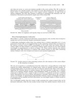
to 1.4 times the hardness of the abrasive [22]. A conceptual graph of wear resistance versus
the ratio of material to abrasive hardness is shown in Figure 11.11. Wear resistance is usually
defined as the reciprocal of wear rates and relative wear resistance is defined as the reciprocal
of wear rate divided by the reciprocal wear rate of a control material.
Natural minerals vary considerably in hardness and abrasivity. The Vickers hardness of
minerals used to define the Mohs scale of hardness have been measured by Tabor [23] and
Mott [24]. The hardness of typical minerals given in Mohs and Vickers is listed in Table 11.1
[23-25].
Silicon carbide which is an artificial mineral has a hardness of 3000 [VHN] (Vickers Hardness

Number) or 30 [GPa]. Quartz (1100 [VHN]) and harder minerals are the main cause of
abrasive wear problems of tough alloy steels which have a maximum hardness of 800 [VHN].
Quartz is particularly widespread in the form of sand and is perhaps the most common agent
of abrasion. The abrasivity of coal is not usually caused by the carbonaceous minerals such as
vitrinite which are relatively soft but by contaminant minerals such as pyrites and hematite
[25]. Identification of the mineral in the grits which causes the excessive abrasive wear is an
TEAM LRN
ABRASIVE, EROSIVE AND CAVITATION WEAR 495
important step in the diagnosis and remedy of this phenomenon. On the other hand,
minerals which are too soft to abrade, e.g. calcite, may still wear a material, but the
mechanisms involved are different, e.g. thermal fatigue [26].


∞
∞
Limit of abrasive wear for
materials with soft phases
or not fully strain hardened
Uniformly hard
materials
Relative wear resistance
100
10
1
0 0.5 1 1.5
Hardness of substrate
Hardness of abrasive
(
(
FIGURE 11.11 Relative abrasive wear resistance versus hardness ratio of worn to abrasive

material.
T
ABLE 11.1 Hardness of typical minerals.


Talc 1 2 3−
Gypsum 2 36 76−
Calcite 3 109 172−
Fluorite 4 190 250−
Apatite 5 566 850−
Orthoclase 6 714 795−
Hematite 6 − 7 1038
Quartz 7 1103 1260−
Pyrite (iron sulphide, cubic form) 7 − 8 1500
Marcasite (iron suphide, orthorhombic form) 7 − 8 1600
8 1200 1648−
9 2060 2720−
10 8000 10 000−Diamond
Topaz or garnet
Corundum
Vitrinite (coal constituent) 4 − 5 294
Substance Mohs’ scale Hardness (VHN)
A more complex constraint is the brittleness of the abrasive. If the grits are too brittle then
they may break up into fine particles, thus minimizing wear [2]. If the abrasive is too tough
then the grits may not fracture to provide the new cutting faces necessary to cause rapid wear
[2,7,8]. The sharp faces of the grits will gradually round-up and the grits will become less
efficient abrasive agents than angular particles [27] as illustrated in Figure 11.12.
TEAM LRN
496 ENGINEERING TRIBOLOGY


123
1
1
234
2
3
4
Very brittle grit
Self-sharpening grit of moderate brittleness
Very tough grit
Initial
angular
shape
Final
rounded
shape
FIGURE 11.12 Effect of grit brittleness and toughness on its efficiency to abrade.
Another factor controlling the abrasivity of a particle is the size and geometry of a grit. The
size of a grit is usually defined as the minimum size of a sphere which encloses the entire
particle. This quantity can be measured relatively easily by sieving a mineral powder through
holes of a known diameter. The geometry of a grit is important in defining how the shape of
the particle differs from an ideal sphere and how many edges or corners are present on the
grit. The non-sphericity of most particles can be described by a series of radii beginning with
the minimum enclosing radius and extending to describe the particle in progressively more
detail as shown in Figure 11.13.

Grit
Minimum size of sphere
enclosing particle
2nd order shape feature

4th or higher
order detail
FIGURE 11.13 Method of defining grit geometry by a series of radii.
TEAM LRN
ABRASIVE, EROSIVE AND CAVITATION WEAR 497
Three parameters are identified as significant in grit description: overall grit size or the
minimum enclosing diameter, the radance, and the roughness of a particle [27]. The radance
is described as the second moment of the radius vector ‘R(θ)’ about the mean radius based on
overall cross sectional area. The roughness is defined as the sum of the squares of higher
order radii above the fourth order of a corresponding Fourier series divided by the mean
radius squared [27]. In other work common abrasives such as SiC, Al
2
O
3
and SiO
2
have been
characterized using aspect ratio (width/length) and perimeter
2
/area shape parameters [63]. It
was found that the erosion rate increased with increasing P
2
/A and decreasing W/L for these
three types of abrasive particles [63].
Recently two new numerical parameters describing the angularity of particles have been
introduced [108-110]. One of the parameters, called ‘spike parameter - linear fit’ (SP), is based
on representing the particle boundary by a set of triangles constructed at different scales and is
calculated in the following manner [108]. A particle boundary is ‘walked’ around at a fixed
step size in a similar manner as used in calculating the boundary fractal dimension [111-113].
The start and the end point at each step is represented by a ‘triangle’ as illustrated in Figure

11.14a [108,109]. It has been assumed that the sharpness and size of these triangles are directly
related to particle abrasivity, i.e. the sharper (smaller apex angle) and larger (perpendicular
height) the triangles are the more abrasive is the particle. The sharpness and size of these
triangles has been described by a numerical parameter called the ‘spike value’, i.e.
sv =
cos
θ
2
h (where: ‘h’ is the perpendicular height of the triangle while ‘θ’ is the apex angle
as shown in Figure 11.14a). For each step around the particle boundary the spike values are
calculated for the largest and sharpest triangles. From the spike values obtained a ‘spike
parameter - linear fit’ is calculated according to the following formula [108,109]:
SP =
Σ

Σ

sv
max
/h
max
/

m
n
(11.17)
where:
sv
max
is max cos

θ
2
h for a given step size;
h
max
is the height at ‘sv
max
’;
m is the number of valid ‘sv’ for a given step size;
n is the number of different step sizes used.
The other parameter, called ‘spike parameter - quadratic fit’ (SPQ), is based on locating a
particle boundary centroid ‘O’ and the average radius circle [110], as illustrated in Figure
11.14b. The areas outside the circle, ‘spikes’, are deemed to be the areas of interest while the
areas inside the circle are omitted. For each protrusion outside the circle, i.e. ‘spike’, the local
maximum radius is found and this point is treated as the spike's apex [110]. The sides of the
‘spike’, which are between the points ‘s-m’ and ‘m-e’, Figure 11.14b, are then represented by
fitting quadratic polynomial functions. Differentiating the polynomials at the ‘m’ point yields
the apex angle ‘θ’ and the spike value ‘sv’, i.e. sv=cosθ/2. From the spike values ‘spike
parameter - quadratic fit’ is then calculated according to the formula [110]:
SPQ = sv
average
(11.18)
One of the advantages of SPQ over SP is that it considers only the boundary features, i.e.
protrusions, which are likely to come in contact with the opposing surface.
It was found that both SP and SPQ correlete well with abrasive wear rates, i.e. two body,
three-body abrasive and erosive wear [109,110,113]. This is illustrated in Figure 11.15 where
TEAM LRN
498 ENGINEERING TRIBOLOGY
the abrasive wear rates obtained with chalk counter-samples are plotted against the
angularity parameters.

Apex
Area
h
Base (step length)
End point
Particle boundary
Start point
Particle
θ
r
mean
s
e
Spike 2
m (apex)
Spike 1
θ
r
local max
O
a)
b)
Figure 11.14 Schematic illustration of particle angularity calculation methods of; a) ‘spike
parameter - linear fit’ (SP) and b) ‘spike parameter - quadratic fit’ (SPQ) (adapted
from [108 and 110]).
0
1
2
3
4

Average wear rate [mm/min]
Spike parameter - linear fit
0.1 0.2 0.3 0.4
gb
g
sic
d
q
ca
ss
0.1
Spike parameter - quadratic fit
gb
ss
g
sic
d
q
ca
0.2 0.3 0.4 0.5 0.6 0.
7
0
a)
b)
Figure 11.15 Relationship between wear rates and particle angularity described by; a) ‘spike
parameter - linear fit’ and b) ‘spike parameter - quadratic fit’ (SPQ) for different
abrasive grit types, i.e. ‘gb’ - glass beads, ‘ss’ - silica sand, ‘g’ - garnet, ‘d’ - natural
industrial diamonds, ‘sic’ - silicon carbide, ‘q’ - crushed quartz and ‘ca’ - crushed
sintered alumina (adapted from [108 and 109]).
It has been found that below 10 [µm] diameter the grits are too small to abrade under certain

conditions [15,19]. The wear rate of an abrasive for constant contact pressure and other
TEAM LRN
ABRASIVE, EROSIVE AND CAVITATION WEAR 499
conditions increases non-linearly with grit diameter up to about 50 [µm] and reaches a
limiting value with grit diameter of about 100 [µm] for most metals [28]. For polymers at high
contact pressures, the wear rate is found to increase with grit diameter up to at least 300 [µm]
[28]. Experimental data of these trends are shown in Figure 11.16.


Wear rate [m
3
/m]
0
5 × 10
-10
0
5 × 10
-10
0
5 × 10
-9
10 × 10
-9
15 × 10
-9
Grit diameter [µm]
0 100 200 300
Polymethylmethacrylate
Nickel
AISI 1095 steel

39.2
19.6
9.8
4.9
39.2
19.6
9.8
4.9
39.2
19.6
9.8
4.9
Normal load [N]
FIGURE 11.16 Effect of abrasive grit diameter and contact pressure on the abrasive wear rate of
a polymer (polymethylmethacrylate, PMMA), nickel and AISI 1095 steel [28].
A fundamental limit to the abrasiveness of particles at extremely small grit diameters is the
surface energy of the abraded material. As grit size decreases the proportion of frictional
energy used for the creation of a new surface increases. For grits within the typical size range
of 5 to 300 [µm], the formation of a new surface consumes less than 0.1% of the energy
absorbed by plastic deformation. With extremely fine grits the formation of a new surface
would absorb a much larger fraction of the available energy [29].
Abrasive Wear Resistance of Materials
The basis of abrasive wear resistance of materials is hardness and it is generally recognized
that hard materials allow slower abrasive wear rates than softer materials. This is supported
by experimental data, an example of which is shown in Figure 11.17. The relative abrasive
wear resistance for a variety of pure metals and alloys after heat treatment is plotted against
the corresponding hardness of the undeformed metal [30-32]. Relative abrasive wear
resistance is defined as wear rate of control material/wear rate of test material. A typical
control material is EN24 steel [e.g. 30-32]. The abrasive material used in these tests was
carborundum with a hardness of 2300 [VHN] and a grit size of 80 [µm]. The tests were

conducted in the two-body mode of abrasive wear with a metallic pin worn against a
carborundum abrasive paper.
TEAM LRN