GOKA: “CHAP05A” — 2006/6/10 — 17:22 — PAGE 42 — #22
42 100 STATISTICAL TESTS
Test 14 Z-test for two correlation coefficients
Object
To investigate the significance of the difference between the correlation coefficients for
a pair of variables occurring from two different samples and the difference between
two specified values ρ
1
and ρ
2
.
Limitations
1. The x and y values originate from normal distributions.
2. The variance in the y values is independent of the x values.
3. The relationships are linear.
Method
Using the notation of the Z-test of a correlation coefficient, we form for the first sample
Z
1
=
1
2
log
e

1 + r
1
1 − r
1

= 1.1513 log

10

1 + r
1
1 − r
1

which has mean µ
Z
1
=
1
2
log
e
[(1 + ρ
1
)/(1 − ρ
1
)] and variance σ
Z
1
= 1/
√
n
1
− 3,
where n
1
is the size of the first sample; Z

2
is determined in a similar manner. The test
statistic is now
Z =
(Z
1
− Z
2
) − (µ
Z
1
− µ
Z
2
)
σ
where σ = (σ
2
Z
1
+ σ
2
Z
2
)
1
2
. Z is normally distributed with mean 0 and with variance 1.
Example
A market research company is keen to categorize a variety of brands of potato crisp based

on the correlation coefficients of consumer preferences. The market research company
has found that if consumers’ preferences for brands are similar then marketing pro-
grammes can be merged. Two brands of potato crisp are compared for two advertising
regions. Panels are selected of sizes 28 and 35 for the two regions and correlation coef-
ficients for brand preferences are 0.50 and 0.30 respectively. Are the two associations
statistically different or can marketing programmes be merged? The calculated Z value
is 0.8985 and the acceptance region for the null hypothesis is −1.96 < Z < 1.96.
So we accept the null hypothesis and conclude that we can go ahead and merge the
marketing programmes. This, of course, assumes that the correlation coefficient is a
good measure to use for grouping market research programmes.
Numerical calculation
n
1
= 28, n
2
= 35, r
1
= 0.50, r
2
= 0.30, α = 0.05
Z
1
= 1.1513 log
10

1 + r
1
1 − r
1


= 0.5493 [Table 4]
GOKA: “CHAP05A” — 2006/6/10 — 17:22 — PAGE 43 — #23
THE TESTS 43
Z
2
= 1.1513 log
10

1 + r
2
1 − r
2

= 0.3095 [Table 4]
σ =

1
n
1
− 3
+
1
n
2
− 3

1
2
= 0.2669
Z =

0.5493 − 0.3095
0.2669
= 0.8985
The critical value at α = 0.05 is 1.96 [Table 1].
Do not reject the null hypothesis.
GOKA: “CHAP05A” — 2006/6/10 — 17:22 — PAGE 44 — #24
44 100 STATISTICAL TESTS
Test 15 χ
2
-test for a population variance
Object
To investigate the difference between a sample variance s
2
and an assumed population
variance σ
2
0
.
Limitations
It is assumed that the population from which the sample is drawn follows a normal
distribution.
Method
Given a sample of n values x
1
, x
2
, , x
n
, the values of
¯x =


x
i
n
and s
2
=

(x
i
−¯x)
2
n − 1
are calculated. To test the null hypothesis that the population variance is equal to σ
2
0
the
test statistic (n −1)s
2
/σ
2
0
will follow a χ
2
-distributkm with n −1 degrees of freedom.
The test may be either one-tailed or two-tailed.
Example
A manufacturing process produces a fixed fluid injection into micro-hydraulic systems.
The variability of the volume of injected fluid is critical and is set at 9 sq ml. A sample
of 25 hydraulic systems yields a sample variance of 12 sq ml. Has the variability of

the volume of fluid injected changed? The calculated chi-squared value is 32.0 and
the 5 per cent critical value is 36.42. So we do not reject the null hypothesis of no
difference. This means that we can still consider the variability to be set as required.
Numerical calculation
¯x = 70, σ
2
0
= 9, n = 25, s
2
= 12, ν = 24
χ
2
= (n − 1)s
2
/σ
2
0
=
24 × 12
9
= 32.0
Critical value x
2
24; 0.05
= 36.42 [Table 5].
Do not reject the null hypothesis. The difference between the variances is not significant.
GOKA: “CHAP05A” — 2006/6/10 — 17:22 — PAGE 45 — #25
THE TESTS 45
Test 16 F-test for two population variances (variance
ratio test)

Object
To investigate the significance of the difference between two population variances.
Limitations
The two populations should both follow normal distributions. (It is not necessary that
they should have the same means.)
Method
Given samples of size n
1
with values x
1
, x
2
, , x
n
1
and size n
2
with values
y
1
, y
2
, , y
n
2
from the two populations, the values of
¯x =

x
i

n
1
, ¯y =

y
i
n
2
and
s
2
1
=

(x
i
−¯x)
2
n
1
− 1
, s
2
2
=

(y
i
−¯y)
2

n
2
− 1
can be calculated. Under the null hypothesis that the variances of the two populations
are equal the test statistic F = s
2
1
/s
2
2
follows the F-distribution with (n
1
− 1, n
2
− 1)
degrees of freedom. The test may be either one-tailed or two-tailed.
Example
Two production lines for the manufacture of springs are compared. It is important that
the variances of the compression resistance (in standard units) for the two production
lines are the same. Two samples are taken, one from each production line and variances
are calculated. What can be said about the two population variances from which the
two samples have been taken? Is it likely that they differ? The variance ratio statistic F
is calculated as the ratio of the two variances and yields a value of 0.36/0.087 = 4.14.
The 5 per cent critical value for F is 5.41. We do not reject our null hypothesis of
no difference between the two population variances. There is no significant difference
between population variances.
Numerical calculation
n
1
= 4, n

2
= 6,

x = 0.4,

x
2
= 0.30, s
2
1
= 0.087

y = 0.06,

y
2
= 1.78, s
2
2
= 0.36
F
3; 5
=
0.36
0.087
= 4.14
Critical value F
3.5; 0.05
= 5.41 [Table 3].
Do not reject the null hypothesis. The two population variances are not significantly

different from each other.
GOKA: “CHAP05A” — 2006/6/10 — 17:22 — PAGE 46 — #26
46 100 STATISTICAL TESTS
Test 17 F-test for two population variances (with
correlated observations)
Object
To investigate the difference between two population variances when there is correlation
between the pairs of observations.
Limitations
It is assumed that the observations have been performed in pairs and that correlation
exists between the paired observations. The populations are normally distributed.
Method
A random sample of size n yields the following pairs of observations
(x
1
, y
1
), (x
2
, y
2
), , (x
n
, y
n
). The variance ratio F is calculated as in Test 16. Also
the sample correlation r is found from
r =

(x

i
−¯x)(y
i
−¯y)


(x
i
−¯x)
2

(y
i
−¯y)
2

1
2
.
The quotient
γ
F
=
F − 1
[(F + 1)
2
− 4r
2
F]
1

2
provides a test statistic with degrees of freedom ν = n −2. The critical values for this
test can be found in Table 6. Here the null hypothesis is σ
2
1
= σ
2
2
, when the population
correlation is not zero. Here F is greater than 1.
Example
A researcher tests a sample panel of television viewers on their support for a particular
issue prior to a focus group, during which the issue is discussed in some detail. The panel
members are then asked the same questions after the discussion. The pre-discussion
view is x and the post-discussion view is y. The question, here, is ‘has the focus group
altered the variability of responses?’
We find the test statistic, F, is 0.796. Table 6 gives us a 5 per cent critical value
of 0.811. For this test, since the calculated value is greater than the critical value, we
do not reject the null hypothesis of no difference between variances. Hence the focus
group has not altered the variability of responses.
GOKA: “CHAP05A” — 2006/6/10 — 17:22 — PAGE 47 — #27
THE TESTS 47
Numerical calculation
n
1
= n
2
= 6,

x = 0.4,


x
2
= 0.30, s
2
1
= 0.087

y = 0.06,

y
2
= 1.78, s
2
2
= 0.36, F =
s
2
2
s
2
1
= 4.14, r = 0.811
γ
F
=
F − 1
[(F + 1)
2
− 4r

2
F]
1
2
=
4.14 − 1
[(5.14)
2
− 4r
2
.4.14]
1
2
=
3.14
[26.42 −16.56 ×0.658]
1
2
= 0.796
α = 0.05, ν = n −2 = 4, r = 0.811 [Table 6].
Hence do not reject the hypothesis of no difference between variances.
The null hypothesis σ
2
1
= σ
2
2
has to be reflected when the value of the test-statistic
equals or exceeds the critical value.
GOKA: “CHAP05A” — 2006/6/10 — 17:22 — PAGE 48 — #28

48 100 STATISTICAL TESTS
Test 18 Hotelling’s T
2
-test for two series of
population means
Object
To compare the results of two experiments, each of which yields a multivariate result.
In other words, we wish to know if the mean pattern obtained from the first experiment
agrees with the mean pattern obtained for the second.
Limitations
All the variables can be assumed to be independent of each other and all variables
follow a multivariate normal distribution. (The variables are usually correlated.)
Method
Denote the results of the two experiments by subscripts A and B. For ease of description
we shall limit the number of variables to three and we shall call these x, y and z. The
number of observations is denoted by n
A
and n
B
for the two experiments. It is necessary
to solve the following three equations to find the statistics a, b and c:
a[(xx)
A
+ (xx)
B
]+b[(xy)
A
+ (xy)
B
]+c[(xz)

A
+ (xz)
B
]
= (n
A
+ n
B
− 2)(¯x
A
−¯x
B
)
a[(xy)
A
+ (xy)
B
]+b[(yy)
A
+ (yy)
B
]+c[(yz)
A
+ (yz)
B
]
= (n
A
+ n
B

− 2)(¯y
A
−¯y
B
)
a[(xz)
A
+ (xz)
B
]+b[(yz )
A
+ (yz)
B
]+c[(zz)
A
+ (zz)
B
]
= (n
A
+ n
B
− 2)(¯z
A
−¯z
B
)
where (xx)
A
=


(x
A
−¯x
A
)
2
, (xy)
A
=

(x
A
−¯x
A
)(y
A
−¯y
A
), and similar definitions
exist for other terms.
Hotelling’s T
2
is defined as
T
2
=
n
A
n

B
n
A
+ n
B
·{a(¯x
A
−¯x
B
) + b(¯y
A
−¯y
B
) + c(¯z
A
−¯z
B
)}
and the test statistic is
F =
n
A
+ n
B
− p − 1
p(n
A
+ n
B
− 2)

T
2
which follows an F-distribution with (p, n
A
+n
B
−p −1) degrees of freedom. Here p
is the number of variables.
Example
Two batteries of visual stimulus are applied in two experiments on young male and
female volunteer students. A researcher wishes to know if the multivariate pattern of
GOKA: “CHAP05A” — 2006/6/10 — 17:22 — PAGE 49 — #29
THE TESTS 49
responses is the same for males and females. The appropriate F statistic is computed
as 3.60 and compared with the tabulated value of 4.76 [Table 3]. Since the computed F
value is less than the critical F value the null hypothesis is of no difference between the
two multivariate patterns of stimulus. So the males and females do not differ in their
responses on the stimuli.
Numerical calculation
n
A
= 6, n
B
= 4, DF = ν = 6 + 4 −4 = 6, α = 0.05
(xx) = (xx)
A
+ (xx)
B
= 19, (yy) = 30, (zz) = 18, (xy) =−6, ν
1

= p = 3
(xz) = 1, (yz) =−7, ¯x
A
=+7, ¯x
B
= 4.5, ¯y
A
= 8, ¯y
B
= 6, ¯z
A
= 6, ¯z
B
= 5
The equations
19a − 6b + c = 20
−6a + 30b −7c = 16
a − 7b + 18c = 8
are satisfied by a = 1.320, b = 0.972, c = 0.749. Thus
T
2
=
6 × 4
10
· (1.320 ×2.5 + 0.972 × 2 +0.749 × 1) = 14.38
F =
6
3 × 8
× 14.38 = 3.60
Critical value F

3.6; 0.0
= 4.76 [Table 3].
Do not reject the null hypothesis.
GOKA: “CHAP05A” — 2006/6/10 — 17:22 — PAGE 50 — #30
50 100 STATISTICAL TESTS
Test 19 Discriminant test for the origin of a p-fold
sample
Object
To investigate the origin of one series of values for p random variates, when one of two
markedly different populations may have produced that particular series.
Limitations
This test provides a decision rule which is closely related to Hotelling’s T
2
-test (Test
18), hence is subject to the same limitations.
Method
Using the notation of Hotelling’s T
2
-test, we may take samples from the two populations
and obtain two quantities
D
A
= a¯x
A
+ b¯y
A
+ c¯z
A
D
B

= a¯x
B
+ b¯y
B
+ c¯z
B
for the two populations. From the series for which the origin has to be traced we can
obtain a third quantity
D
S
= a¯x
S
+ b¯y
S
+ c¯z
S
.
If D
A
−D
S
< D
B
−D
S
we say that the series belongs to population A, but if D
A
−D
S
>

D
B
− D
S
we conclude that population B produced the series under consideration.
Example
A discriminant function is produced for a collection of pre-historic dog bones. A new
relic is found and the appropriate measurements are taken. There are two ancient pop-
ulations of dog A or B to which the new bones could belong. To which population do
the new bones belong? This procedure is normally performed by statistical computer
software. The D
A
and D
B
values as well as the D
S
value are computed. The D
S
value
is closer to D
A
and so the new dog bone relic belongs to population A.
Numerical calculation
a = 1.320, b = 0.972, c = 0.749
¯x
A
= 7, ¯y
A
= 8, ¯z
A

= 6, ¯x
B
= 4.5, ¯y
B
= 6, ¯z
B
= 5
D
A
= 1.320 × 7 +0.972 × 8 + 0.749 ×6 = 21.510
D
B
= 1.320 × 4.5 +0.972 × 6 + 0.749 ×5 = 15.517
If ¯x
S
= 6, ¯y
S
= 6 and ¯z
S
= 7, then
D
S
= 1.320 × 6 +0.972 × 6 + 0.749 ×7 = 18.995
D
A
− D
S
= 21.510 − 18.995 = 2.515
D
B

− D
S
= 15.517 − 18.995 =−3.478
D
S
lies closer to D
A
. D
S
belongs to population A.
GOKA: “CHAP05A” — 2006/6/10 — 17:22 — PAGE 51 — #31
THE TESTS 51
Test 20 Fisher’s cumulant test for normality of a
population
Object
To investigate the significance of the difference between a frequency distribution based
on a given sample and a normal frequency distribution with the same mean and the
same variance.
Limitations
The sample size should be large, say n > 50. If the two distributions do not have the
same mean and the same variance then the w/s-test (Test 33) can be used.
Method
Sample moments can be calculated by
M
r
=
n

i=1
x

r
i
or M
r
=
n

i=1
x
n
i
f
i
where the x
i
are the interval midpoints in the case of grouped data and f
i
is the frequency.
The first four sample cumulants (Fisher’s K-statistics) are
K
1
=
M
1
n
K
2
=
nM
2

− M
2
1
n(n − 1)
K
3
=
n
2
M
3
− 3nM
2
M
1
+ 2M
3
1
n(n − 1)(n −2)
K
4
=
(n
3
+ n
2
)M
4
− 4(n
2

+ n)M
3
M
1
− 3(n
2
− n)M
2
2
+ 12M
2
M
2
1
− 6M
4
1
n(n − 1)(n −2)(n −3)
To test for skewness the test statistic is
u
1
=
K
3
(K
2
)
3
2
×


n
6

1
2
which should follow a standard normal distribution.
To test for kurtosis the test statistic is
u
2
=
K
4
(K
2
)
2
×

n
24

1
2
which should follow a standard normal distribution.
GOKA: “CHAP05A” — 2006/6/10 — 17:22 — PAGE 52 — #32
52 100 STATISTICAL TESTS
A combined test can be obtained using the test statistic
χ
2

=

K
3
(K
2
)
3
2
×

n
6

1
2

2
+

K
4
(K
2
)
2
×

n
24


1
2

2
which will approximately follow a χ
2
-distribution with two degrees of freedom.
Example
Example A
A large sample of 190 component measurements yields the following calculations (see
table). Do the sample data follow a normal distribution? The test for skewness is a u
1
statistic of 0.473 and the critical value of the normal test statistic is 1.96. Since u
1
is
less than this critical value we do not reject the null hypothesis of no difference. So for
skewness the data are similar to a normal distribution. For kurtosis we have u
2
statistic
of 0.474 and, again, a critical value of 1.96. So, again, we accept the null hypothesis;
kurtosis is not significantly different from that of a normal distribution with the same
mean and variance. The combined test gives a calculated chi-squared value 0.449 which
is smaller than the 5 per cent critical value of 5.99. So we conclude that the data follow
a normal distribution.
Example B
We calculate the values of skewness and kurtosis together with their respective standard
deviations and produce:
u
1

= skewness/sd= 0.477
u
2
= kurtosis/sd= 0.480
Table 7 gives (for sample sizes 200 and 175) critical values for u
1
of 0.282 to 0.301
and for u
2
of 0.62 to 0.66. So, again, we accept the null hypothesis.
Numerical calculation
Example A

f = n = 190,

fx = 151,

fx
2
= 805,

fx
3
= 1837,

fx
4
= 10 753
i.e. M
1

= 151, M
2
= 805, M
3
= 1837, M
4
= 10 753
K
2
=
(190 ×805) −(151)
2
190 ×189
= 3.624310
K
3
=
(190)
2
× 1837 −3 ×190 × 805 ×151 +2(151)
3
190 ×189 ×188
= 0.5799445
K
4
=
2 795 421 924
190 ×189 ×188 × 187
= 2.214280
GOKA: “CHAP05A” — 2006/6/10 — 17:22 — PAGE 53 — #33

THE TESTS 53
Test for skewness
u
1
=
0.579945
3.62431
√
3.624310
× 5.6273 = 0.08405 × 5.6273 = 0.473
The critical value at α = 0.05 is 1.96.
Do not reject the null hypothesis [Table 1].
Test for kurtosis
u
2
=
2.214279
(3.62431)
2
×

190
24

1
2
= 0.1686 × 2.813657 = 0.474
The critical value at α = 0.05 is 1.96.
Do not reject the null hypothesis [Table 1].
Combined test

χ
2
= (0.473)
2
+ (0.474)
2
= 0.2237 + 0.2250 = 0.449
which is smaller than the critical value 5.99 [Table 5].
Example B
Let skewness = g
1
=
K
3
K
2
√
K
2
=
0.579945
3.624310
√
3.624310
= 0.084052
kurtosis = g
2
=
K
4

K
2
2
=
2.214279
(3.624310)
2
= 0.168570
standard deviation σ(g
1
) =

6n(n − 1)
(n − 2)(n +1)(n +3)
=

6 × 190 ×189
188 × 191 ×193
=
√
0.0310898 = 0.176323
standard deviation σ(g
2
) =

24n(n − 1)
2
(n − 3)(n − 2)(n + 3)(n +5)
=


24 × 190 ×189
2
187 × 188 ×193 × 195
= 0.350872
Here u
1
=
0.084052
0.176323
= 0.477, u
2
=
0.168570
0.350872
= 0.480.
Critical values for g
1
lie between 0.282 (for 200) and 0.301 (for 175) [Table 7].
The right-side critical value for g
2
lies between 0.62 and 0.66 [Table 7].
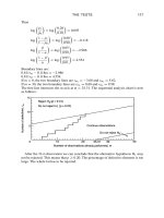
Hence the null hypothesis should not be rejected.
GOKA: “CHAP05A” — 2006/6/10 — 17:22 — PAGE 54 — #34
54 100 STATISTICAL TESTS
Test 21 Dixon’s test for outliers
Object
To investigate the significance of the difference between a suspicious extreme value
and other values in the sample.
Limitations
1. The sample size should be greater than 3.

2. The population which is being sampled is assumed normal.
Method
Consider a sample of size n, where the sample is arranged with the suspect value in
front, its nearest neighbour next and then the following values arranged in ascending (or
descending) order. The order is determined by whether the suspect value is the largest
or the smallest. Denoting the ordered series by x
1
, x
2
, , x
n
, the test statistic r where
r = (x
2
− x
1
)/(x
n
− x
1
) if 3 < n  7,
r = (x
2
− x
1
)/(x
n−1
− x
1
) if 8  n  10,

r = (x
3
− x
1
)/(x
n−1
− x
1
) if 11  n  13,
r = (x
3
− x
1
)/(x
n−2
− x
1
) if 14  n  25.
Critical values for r can be obtained from Table 8. The null hypothesis that the outlier
belongs to the sample is rejected if the observed value of r exceeds the critical value.
Example
As part of a quality control programmed/implementation small samples are taken, at
regular intervals, for a number of processes. On several of these processes there is
the potential for inaccuracies occurring in the measurements that are taken due to the
complexity of the measuring process and the inexperience of the process workers. One
such sample of size 4 is tested for potential outliers and the following are produced:
x
1
= 326, x
2

= 177, x
3
= 176, x
4
= 157.
Dixon’s ratio yields r = 0.882.
The critical value at the 5 per cent level from Table 8 is 0.765, so the calculated value
exceeds the critical value. We thus reject the null hypothesis that the outlier belongs
to the sample. Thus we need to re-sample and measure again or only use three sample
values in this case.
Numerical calculation
x
1
, = 326, x
2
= 177, x
3
= 176, x
4
= 157, n = 4
Here r =
x
2
− x
1
x
n
− x
1
=

177 − 326
157 − 326
= 0.882
The critical value at α = 0.05 is 0.765 [Table 8].
The calculated value exceeds the critical value.
Hence reject the null hypothesis that the value x
1
comes from the same population.
GOKA: “CHAP05A” — 2006/6/10 — 17:22 — PAGE 55 — #35
THE TESTS 55
Test 22 F-test for K population means (analysis of
variance)
Object
To test the null hypothesis that K samples are from K populations with the same mean.
Limitations
It is assumed that the populations are normally distributed and have equal variances. It
is also assumed that the samples are independent of each other.
Method
Let the jth sample contain n
j
elements ( j = 1, , K). Then the total number of
elements is
N =
K

j=1
n
j
The ith element of the jth sample can be denoted by x
ij

(i = 1, , n
j
), and the mean
of the jth sample becomes
x
·j
=
n

j=1
x
ij
/n
j
The variance of the observations with respect to their own sample means becomes
s
2
1
=

j

i
(x
ij
− x
·j
)
2
N − K

or equivalently, denoting the total sum of squares of all the observations as s
2
T
,
(s
2
T
− s
2
2
)/(N − K)
with N − K degrees of freedom. Similarly, the variance of the sample means with
respect to the grand mean becomes
s
2
2
=

j
n
j
(x
·j
− x
··
)
2
K − 1
where
x

··
=
1
K

i

j
x
ij
and s
2
2
has K − 1 degrees of freedom.
GOKA: “CHAP05A” — 2006/6/10 — 17:22 — PAGE 56 — #36
56 100 STATISTICAL TESTS
The test statistic is F = s
2
2
/s
2
1
, which follows the F-distribution with (K −1, N −K)
degrees of freedom. A one-tailed test is carried out as it is necessary to ascertain whether
s
2
2
is larger than s
2
1

.
Example
A petroleum company tests three additives on its premium unleaded petrol to assess their
effect on petrol consumption. The company uses a basic car of a particular make and
model with cars randomly allocated to treatments (additives). An analysis of variance
compares the effect of the additives on petrol consumption. Since the calculated F
statistic at 37 is greater than the tabulated value of 4.26 the variance between additives
is greater than the variance within additives. The additives have an effect on petrol
consumption.
Numerical calculation
K = 3, N = 12, n
1
= 3, n
2
= 5, n
3
= 4, α = 0.05
n
1

i=1
x
i1
= 53.5,
n
2

i=1
x
i2

= 102.5,
n
3

i=1
x
i3
= 64.4
T = 53.5 +102.5 +64.4 = 220.4
x
1
= 17.83, x
2
= 20.50, x
3
= 16.10, x

= T/N = 18.37
T
2
/N = 4048.01
s
2
T
=

n
1

i=1

x
2
i1
+
n
2

i=1
x
2
i2
+
n
3

i=1
x
2
i3

−
T
2
N

=[(954.43 + 2105.13 +1037.98) − 4048.01]
= 4097.54 − 4048.01
= 49.53
s
2

2
= 44.17
F
2,9
=
s
2
2
/(K − 1)
s
2
1
/(N − K)
=
s
2
2
/(K − 1)
(s
2
T
− s
2
2
)/(N − K)
=
44.17/2
(49.53 − 44.17)/9
 37
Critical value F

2,9; 0.05
= 4.26 [Table 3].
The calculated value is greater than the critical value.
The variance between the samples is significantly larger than the variance within the
samples.
GOKA: “CHAP05A” — 2006/6/10 — 17:22 — PAGE 57 — #37
THE TESTS 57
Test 23 The Z-test for correlated proportions
Object
To investigate the significance of the difference between two correlated proportions in
opinion surveys. It can also be used for more general applications.
Limitations
1. The same people are questioned both times on a yes–no basis.
2. The sample size must be quite large.
Method
N people respond to a yes–no question both before and after a certain stimulus. The
following two-way table can then be built up:
First poll
Yes No
Second Yes a b
poll No c d
N
To decide whether the stimulus has produced a significant change in the proportion
answering ‘yes’, we calculate the test statistic
Z =
b − c
Nσ
where
σ =


(b + c) −(b − c)
2
/N
N(N − 1)
.
Example
Sampled panels of potential buyers of a financial product are asked if they might buy
the product. They are then shown a product advertisement of 30 seconds duration and
asked again if they would buy the product. Has the advertising stimulus produced a
significant change in the proportion of the panel responding ‘yes’?
We have
First poll
Yes No
Second
Yes 30 15
poll
No 9 51
GOKA: “CHAP05A” — 2006/6/10 — 17:22 — PAGE 58 — #38
58 100 STATISTICAL TESTS
which yields the test statistic Z = 1.23. The 5 per cent critical value from the normal
distribution is 1.96. Since 1.23 is less than 1.96 we do not reject the null hypothesis of
no difference. The advertisement does not increase the proportion saying ‘yes’. Notice
that we have used a one-tailed test, here, because we are only interested in an increase,
i.e. a positive effect of advertising.
Numerical calculation
a = 30, b = 15, c = 9, d = 51, N = 105
The null hypothesis is that there is no apparent change due to the stimulus.
The difference in proportion is
b − c
N

=
15
105
−
9
105
=
6
105
= 0.0571
σ =

(15 + 9) − (15 − 9)
2
/105
105 × 104
= 0.0465
Z =
0.0571
0.0465
= 1.23
The critical value at α = 0.05 is 1.96 [Table 1].
The calculated value is less than the critical value.
Do not reject the null hypothesis.
GOKA: “CHAP05A” — 2006/6/10 — 17:22 — PAGE 59 — #39
THE TESTS 59
Test 24 χ
2
-test for an assumed population variance
Object

To investigate the significance of the difference between a population variance σ
2
and
an assumed value σ
2
0
.
Limitations
It is assumed that the sample is taken from a normal population.
Method
The sample variance
s
2
=
n

i=1
(x
i
−¯x)
2
n − 1
is calculated. The test statistic is then
χ
2
=
s
2
σ
2

0
(n − 1)
which follows a χ
2
-distribution with n − 1 degrees of freedom.
Example
An engineering process has specified variance for a machined component of 9 square
cm. A sample of 25 components is selected at random from the production and the
mean value for a critical dimension on the component is measured at 71 cm with
sample variance of 12 square cm. Is there a difference between variances? A calculated
chi-squared value of 32 is less than the tabulated value of 36.4 suggesting no difference
between variances.
Numerical calculation
n = 25, ¯x = 71, s
2
= 12, σ
2
0
= 9
H
0
: σ
2
= σ
2
0
, H
1
: σ
2

= σ
2
0
χ
2
= 24 ×
12
9
= 32
Critical value χ
2
24; 0.05
= 36.4 [Table 5].
Do not reject the null hypothesis. The difference between the variances is not significant.
GOKA: “CHAP05A” — 2006/6/10 — 17:22 — PAGE 60 — #40
60 100 STATISTICAL TESTS
Test 25 F-test for two counts (Poisson distribution)
Object
To investigate the significance of the difference between two counted results (based on
a Poisson distribution).
Limitations
It is assumed that the counts satisfy a Poisson distribution and that the two samples
were obtained under similar conditions.
Method
Let µ
1
and µ
2
denote the means of the two populations and N
1

and N
2
the two counts.
To test the hypothesis µ
1
= µ
2
we calculate the test statistic
F =
N
1
N
2
+ 1
which follows the F-distribution with (2(N
2
+1),2N
1
) degrees of freedom. When the
counts are obtained over different periods of time t
1
and t
2
, it is necessary to compare
the counting rates N
1
/t
1
and N
2

/t
2
. Hence the appropriate test statistic is
F =
1
t
1
(N
1
+ 0.5)
1
t
2
(N
1
+ 0.5)
which follows the F-distribution with (2N
1
+ 1, 2N
2
+ 1) degrees of freedom.
Example
Two automated kiln processes (producing baked plant pots) are compared over their
standard cycle times, i.e. 4 hours. Kiln 1 produced 13 triggered process corrections and
kiln 2 produced 3 corrections. What can we say about the two kiln mean correction
rates, are they the same? The calculated F statistic is 3.25 and the critical value from
Table 3 is 2.32. Since the calculated value exceeds the critical value we conclude that
there is a statistical difference between the two counts. Kiln 1 has a higher error rate
than kiln 2.
Numerical calculation

N
1
= 13, N
2
= 3, t
1
= t
2
f
1
= 2(N
2
+ 1) = 2(3 + 1) = 8, f
2
= 2N
1
= 2 × 13 = 26
F =
N
1
N
2
+ 1
=
13
3 + 1
= 3.25
Critical value F
8,26; 0.05
= 2.32 [Table 3].

The calculated value exceeds the table value.
Hence reject the null hypothesis.
GOKA: “CHAP05B” — 2006/6/10 — 17:22 — PAGE 61 — #1
THE TESTS 61
Test 26 F-test for the overall mean of K
subpopulations (analysis of variance)
Object
To investigate the significance of the difference between the overall mean of K sub-
populations and an assumed value µ
0
for the population mean. Two different null
hypotheses are tested; the first being that the K subpopulations have the same mean
(µ
1
= µ
2
=···=µ
K
) and the second that the overall mean is equal to the assumed
value (µ = µ
0
).
Limitations
The K samples from the subpopulations are independent of each other. The subpopu-
lations should also be normally distributed and have the same variance.
Methods
Method A
To test H
0
: µ

1
= µ
2
=···=µ
K
, we calculate the test statistic
F =
s
2
1
/(K − 1)
s
2
2
/(N − K)
where N is the total number of observations in the K samples, n
j
is the number of
observations in the jth sample,
s
2
1
=

j
n
j
(x
·j
− x

··
)
2
s
2
2
=

i

j
(x
ij
− x
·j
)
2
⎫
⎪
⎪
⎬
⎪
⎪
⎭
i = 1, , n
j
, j = 1, , K,
and x
ij
is the ith observation in the jth sample

x
·j
=
1
n
j

i
x
ij
x
··
=
1
N

i

j
x
ij
The value of F should follow the F-distribution with (K −1, N −K) degrees of freedom.
Method B
To test H
0
: µ = µ
0
, we calculate the test statistic
F =
N(x

··
− µ
0
)
2
s
2
1
/(K − 1)
which should follow the F-distribution with (1, K − 1) degrees of freedom.
GOKA: “CHAP05B” — 2006/6/10 — 17:22 — PAGE 62 — #2
62 100 STATISTICAL TESTS
Example
A nutritional researcher wishes to test the palatability of six different formulations
of vitamin/mineral supplement which are added to children’s food. They differ only
in their taste. Are they equally palatable? Do they, overall, produce a given average
consumption of food? In a trial, six groups each of five children are given the different
formulations. The first calculated F value of 4.60 tests for equality of palatability. Since
this exceeds the tabulated value of 2.62 the null hypothesis of no difference is rejected.
The formulations do affect the palatability of the food eaten since different quantities
are eaten. The second F value of 2.01, since it is less than the tabulated value of 6.61,
suggests that the formulations, if used together over a period of time, will not affect
consumption.
Numerical calculation
n
1
= n
2
= n
3

= n
4
= n
5
= n
6
= 5, K = 6, N = 30, µ
0
= 1500
x
·1
= 1505, x
·2
= 1528, x
·3
= 1564, x
·4
= 1498, x
·5
= 1600, x
·6
= 1470
¯x
··
= 9165/6 = 1527.5
s
2
1
/5 = 11 272, s
2

2
/24 = 2451, s
2
T
= 3972
N(x
··
− µ
0
)
2
= 22 687.5
(a) F = 11 272/2451 = 4.60.
Critical value F
5, 24; 0.05
= 2.62 [Table 3].
Reject the null hypothesis.
(b) F = 22 687.5/11 272 = 2.01.
Critical value F
1,5; 0.05
= 6.61 [Table 3].
Do not reject the null hypothesis.
GOKA: “CHAP05B” — 2006/6/10 — 17:22 — PAGE 63 — #3
THE TESTS 63
Test 27 F-test for multiple comparison of contrasts
between K population means
Object
This test is an extension of the preceding one, to investigate which particular set of
mean values or linear combination of mean values shows differences with the other
mean values.

Limitations
As for the preceding test, with the addition that the comparisons to be examined should
be decided on at or before the start of the analysis.
Method
With the notation as before, we must define a contrast as a linear function of the means
λ =
K

j=1
a
j
µ
j
under the condition that

K
j=1
a
j
= 0.
The test statistic becomes
F =
1
s
2
⎛
⎝
K

j=1

a
j
x
·j
⎞
⎠
2
K

j=1
a
2
j
/n
j
(see Test 26) which should follow the F-distribution with (1, N −K) degrees of freedom.
Here,
s
2
=
K

j=1
n
j

i=1
(x
ij
)

2
−
K

j=1
n
j
¯x
2
j
N − K
.
For simple differences of the type ¯x
·i
−¯x
·j
the test statistic becomes
F =
(¯x
·i
−¯x
·j
)

1
n
i
+
1
n

j

s
2
GOKA: “CHAP05B” — 2006/6/10 — 17:22 — PAGE 64 — #4
64 100 STATISTICAL TESTS
Example
Three different filters are used on an artificial lighting system for plant production. An
agricultural researcher wishes to test whether any filter is better than the others in terms
of the yield of a crop. He designs and conducts his experiment and performs the F test.
He compares each plant yield with the others.
For comparing filter 1 with filter 2 his calculated F value is 0.646; for comparing
filter 1 with filter 3 his F value is 36.78 and for comparing filter 2 with filter 3 his
F value is 39.90. So it appears that filter 1 and filter 2 are similar in relation to plant
growth but there is a difference between filter 1 and filter 3 and filter 2 and filter 3.
Numerical calculation
n
1
= 6, n
2
= 4, n
3
= 2, N = 12, K = 3, ν
1
= 1, ν
2
= 9
¯x
·1
= 2.070, ¯x

·2
= 2.015, ¯x
·3
= 2.595, ¯x = 2.139

i

j
x
2
ij
= 55.5195,

n
j
¯x
2
j
= 55.41835
λ
1
= µ
1
− µ
2
, λ
2
= µ
1
− µ

3
, λ
3
= µ
2
− µ
3
(contrasts)
¯x
·1
−¯x
·2
= 0.055
¯x
·1
−¯x
·3
=−0.525
¯x
·2
−¯x
·3
=−0.580
(x
·1
− x
·2
)
2


1
n
1
+
1
n
2

=
(0.055)
2

1
6
+
1
4

= 0.00726
(x
·1
− x
·3
)
2

1
n
1
+

1
n
3

=
(−0.525)
2

1
6
+
1
2

= 0.4134
(x
·2
− x
·3
)
2

1
n
2
+
1
n
3


=
(−0.580)
2

1
4
+
1
2

= 0.4485
s
2
=
55.5195 − 55.41835
9
=
0.10115
9
= 0.01124
F
1
=
0.00726
0.01124
= 0.646, F
2
=
0.4134
0.01124

= 36.78, F
3
=
0.4485
0.01124
= 39.90
Critical value F
1,9;0.05
= 5.12 [Table 3]. Both F
2
and F
3
are larger than 5.12. There
is no significant difference between the means for group 1 and group 2, but there is a
significant difference between group 3 and groups 1 and 2.
GOKA: “CHAP05B” — 2006/6/10 — 17:22 — PAGE 65 — #5
THE TESTS 65
Test 28 Tukey test for multiple comparison of K
population means (unequal sample sizes)
Object
To investigate the significance of all possible differences between K population means.
Limitations
The K populations are normally distributed with equal variances.
Method
Consider samples of size n
1
, n
2
, , n
K

from the K populations. From Table 9 the
critical values of q can be found using degrees of freedom
ν =
⎛
⎝
K

j=1
n
j
⎞
⎠
− K.
The total variance of the samples is now calculated from
s
2
=
K

j=1
(n
j
− 1) · s
2
j
N − K
where s
2
j
is the variance of the jth sample and N is the total sample size. Finally, a limit

W is calculated
W =
qs
n
1
2
where q (=w/s) is the Studentized range and
n =
K

1
n
1
+
1
n
2
+···+
1
n
K

.
If this limit W is exceeded by the absolute difference between any two sample means,
then the corresponding population means differ significantly.
Example
Five different grades of grit used for agricultural purposes are produced. A filling
machine fills small sacks with a nominal 500 gm weight, although more is usually dis-
pensed. An agricultural merchant is concerned that the weight does not differ between
grades. He uses Tukey’s test to compare all five grades and produces a critical limit of

W at 55.3. Since the largest difference grades is 35.8 and is less than 55.17 he concludes
that the grades do not differ with respect to weight.
GOKA: “CHAP05B” — 2006/6/10 — 17:22 — PAGE 66 — #6
66 100 STATISTICAL TESTS
Numerical calculation
n
1
= n
2
= n
3
= n
4
= n
5
= 5, K = 5, N = 25
s
2
1
= 406.0, s
2
2
= 574.8, s
2
3
= 636.8, s
2
4
= 159.3, s
2

5
= 943.2
¯x
1
= 534.0, ¯x
2
= 536.4, ¯x
3
= 562.6, ¯x
4
= 549.4, ¯x
5
= 526.8
s
2
=
2720.1
5
= 544.02, s = 23.32, ν = 25 −5 = 20
Critical value for q for K = 5, and ν = 20 at α = 0.05 is 5.29 [Table 9].
W =
5.29 × 23.32
√
5
= 55.17
The largest difference between the sample means is 562.6 −526.8 = 35.8 which is less
than 55.17. Hence the population means do not differ significantly.