100 STATISTICAL TESTS phần 4 doc
Bạn đang xem bản rút gọn của tài liệu. Xem và tải ngay bản đầy đủ của tài liệu tại đây (147.82 KB, 25 trang )
GOKA: “CHAP05B” — 2006/6/10 — 17:22 — PAGE 67 — #7
THE TESTS 67
Test 29 The Link–Wallace test for multiple
comparison of K population means
(equal sample sizes)
Object
To investigate the significance of all possible differences between K population means.
Limitations
1. The K populations are normally distributed with equal variances.
2. The K samples each contain n observations.
Method
The test statistic is
K
L
=
nw(¯x)
k
i=1
w
i
(x)
where w
i
(x) is the range of the x values for the ith sample
w(¯x) is the range of the sample means
n is the sample size.
The null hypothesis µ
1
= µ
2
=···=µ
K
is rejected if the observed value of K
L
is
larger than the critical value obtained from Table 10.
Example
Three advertising theme tunes are compared using three panels to assess their pleasure,
using a set of scales. The test statistic D is computed as 2.51, and then the three
differences between the ranges of means are also calculated. Tunes 3 and 2 differ as do
tunes 3 and 1, but tunes 1 and 2 do not.
Numerical calculation
n = 8, w
1
(x) = 7, w
2
(x) = 6, w
3
(x) = 4, K = 3
w
1
(¯x) = 4.750, w
2
(¯x) = 4.625, w
3
(¯x) = 7.750
K
L
=
nw(¯x)
k
i=1
w
i
(x)
=
8(7.750 −4.625)
7 + 6 +4
= 1.47
Critical value K
8,3;0.05
= 1.18 [Table 10].
Reject the null hypothesis of equal means.
GOKA: “CHAP05B” — 2006/6/10 — 17:22 — PAGE 68 — #8
68 100 STATISTICAL TESTS
Using K
8,3;0.05
= 1.18, the critical value for the sample mean differences is
D =
1.18
w
i
(x)
n
=
1.18 × 17
8
= 2.51
Since w
1
(¯x) −w
2
(¯x) = 0.125 (less than D)
w
3
( ¯w) − w
2
(¯x) = 3.125 (greater than D)
w
3
(¯x) −w
1
(¯x) = 3.00 (greater than D)
reject the null hypothesis µ
1
= µ
3
and µ
2
= µ
3
.
GOKA: “CHAP05B” — 2006/6/10 — 17:22 — PAGE 69 — #9
THE TESTS 69
Test 30 Dunnett’s test for comparing K treatments
with a control
Object
To investigate the significance of the differences, when several treatments are compared
with a control.
Limitations
1. The K +1 samples, consisting of K treatments and one control, all have the same
size n.
2. The samples are drawn independently from normally distributed populations with
equal variances.
Method
The variance within the K + 1 groups is calculated from
S
2
W
=
S
2
0
+ S
2
1
+···+S
2
K
(K − 1)(n − 1)
where S
2
0
is the sum of squares of deviations from the group mean for the control group
and S
2
j
is a similar expression for the jth treatment group. The standard deviation of the
differences between treatment means and control means is then
S(
¯
d) =
2S
2
W
/n
The quotients
D
j
=
¯x
j
−¯x
0
S(
¯
d)
( j = 1, 2, , K)
are found and compared with the critical values of |D
j
| found from Table 11. If
an observed value is larger than the tabulated value, one may conclude that the
corresponding difference in means between treatment j and the control is significant.
Example
Four new topical treatments for athlete’s foot are compared with a control, which is
the current accepted treatment. Patients are randomly allocated to each treatment and
the number of days to clear up of the condition is the treatment outcome. Do the new
treatments differ from the control? The critical value, D, from Table 11 is 2.23 and all
standardized differences are compared. Treatment 1 shows a difference from control
which is significant. This treatment results in a longer time to clear up.
GOKA: “CHAP05B” — 2006/6/10 — 17:22 — PAGE 70 — #10
70 100 STATISTICAL TESTS
Numerical calculation
K = 4, n = 10, ¯x
0
= 14.5, ¯x
1
= 25.0, ¯x
2
= 15.7, ¯x
3
= 18.1, ¯x
4
= 21.9
S
2
0
= 261.0, S
2
1
= 586.0, S
2
2
= 292.6, S
2
3
= 320.4, S
2
4
= 556.4
S
2
W
=
261 + 586 +292.6 +320.4 +556.4
(4 − 1)(10 −1)
= 74.681
S(
¯
d) =
2S
2
W
/n =
2 ×74.681
10
1
2
= 3.865
Critical value D
4,45;0.05
= 2.23 [Table 11].
D
1
= 2.72, D
2
= 0.31, D
3
= 0.93, D
4
= 1.91
The value of D
1
is larger than the critical value. Hence D
1
is significantly different
from the control value.
GOKA: “CHAP05B” — 2006/6/10 — 17:22 — PAGE 71 — #11
THE TESTS 71
Test 31 Bartlett’s test for equality of K variances
Object
To investigate the significance of the differences between the variances of K normally
distributed populations.
Limitations
It is assumed that all the populations follow a normal distribution.
Method
Samples are drawn from each of the populations. Let s
2
j
denote the variance of a sample
of n
j
items from the jth population ( j = 1, , K). The overall variance is defined by
s
2
=
K
j=1
(n
j
− 1) · s
2
j
K
j=1
(n
j
− 1)
.
The test statistic is
B =
2.30259
C
(n
j
− 1) log s
2
−
(n
j
− 1) log s
2
j
where
C = 1 +
1
3(K + 1)
1
(n
j
− 1)
−
1
(n
j
− 1)
and log
e
10 = 2.30259.
Case A (n
j
> 6)
B will approximate to a χ
2
-distribution with K − 1 degrees of freedom. The null
hypothesis of equal variances is rejected if B is larger than the critical value.
Case B (n
j
6)
The test statistic becomes BC = M and this should be referred to Table 12. When the
value of M exceeds the tabulated value, the null hypothesis can be rejected.
Example
A bank of four machining heads is compared in relation to the variability of the end
machined components. A quality engineer has collected a randomized sequence of
components and measured the relevant component dimensions. In his first test he has
large samples and computes the test statistic B, which is 7.31. This is less than the
critical value of 7.81 from Table 5. He so concludes that the variabilities for the four
machine heads are the same.
GOKA: “CHAP05B” — 2006/6/10 — 17:22 — PAGE 72 — #12
72 100 STATISTICAL TESTS
In a subsequent test of equality of variances the engineer takes smaller samples which
necessitate his use of tables for comparison. In this case his sample values produce an
M value which is less than the tabulated value of 9.21 from Table 12. So again he
concludes that the variances are the same.
Numerical calculation
Example A
n
1
= 31, n
2
= 15, n
3
= 20, n
4
= 42, K = 4
s
2
1
= 5.47, s
2
2
= 4.64, s
2
3
= 11.47, s
2
4
= 11.29
s
2
=
910
104
= 8.75, log s
2
= 0.94201, C = 1.01
(n
j
− 1) log s
2
= 97.9690,
(n
j
− 1) log s
2
j
= 94.7630
B =
1
1.01
[2.30259(97.9690 −94.7630)]=
7.38
1.01
= 7.31
Critical value χ
2
3;0.05
= 7.81 [Table 5].
Hence the null hypothesis is not rejected.
Example B
n
1
= 3, n
2
= 3, n
3
= 3, n
4
= 4
s
2
1
= 6.33, s
2
2
= 1.33, s
2
3
= 4.33, s
2
4
= 4.33
Pooled variance s
2
=
(12.66 + 2.66 +8.66 +12.99)
2 +2 +2 + 3
= 4.11
Further
M = 2.30259{9 log 4.11 − 2 log 6.33 − 2 log 1.33 − 2 log 4.33 −3 log 4.33}
= 2.30259{9 × 0.6138 − 2 ×0.8014 −2 × 0.1239 − 2 × 0.6365
− 3 × 0.6365}=1.131
C =
1
2
+
1
2
+
1
2
+
1
3
−
1
9
= 1.7222
The critical value of M for α = 0.05, K = 4 is 9.21 [Table 12]; even for C = 2.0. Do
not reject the null hypothesis.
GOKA: “CHAP05B” — 2006/6/10 — 17:22 — PAGE 73 — #13
THE TESTS 73
Test 32 Hartley’s test for equality of K variances
Object
To investigate the significance of the differences between the variances of K normally
distributed populations.
Limitations
1. The populations should be normally distributed.
2. The sizes of the K samples should be (approximately) equal.
Method
Samples are drawn from each of the populations. The test statistic is F
max
= s
2
max
/s
2
min
where s
2
max
is the largest of the K sample variances and s
2
min
is the smallest of the K
sample variances.
Critical values of F
max
can be obtained from Table 13. If the observed ratio exceeds
this critical value, the null hypothesis of equal variances should be rejected.
Example
Four types of spring are tested for their response to a fixed weight since they are used
to calibrate a safety shut-off device. It is important that the variability of responses
is equal. Samples of responses to a weight on each spring are taken. The Hartley F
statistic is calculated to be 2.59 and is compared with the critical tabulated value of
2.61 [Table 13]. Since the calculated statistic is less than the tabulated value the null
hypothesis of equal variances is accepted.
Numerical calculation
n
1
= n
2
= n
3
= n
4
= 30, K = 4
s
2
1
= 16.72, s
2
2
= 36.27, s
2
3
= 14.0, s
2
4
= 15.91
F =
36.27
14.0
= 2.59
The critical value of F
max
, at a 5 per cent level of significance, for n = 30, K = 4is
2.61 [Table 13].
Hence do not reject the null hypothesis.
GOKA: “CHAP05B” — 2006/6/10 — 17:22 — PAGE 74 — #14
74 100 STATISTICAL TESTS
Test 33 The w/s-test for normality of a population
Object
To investigate the significance of the difference between a frequency distribution based
on a given sample and a normal frequency distribution.
Limitations
This test is applicable if the sample is taken from a population with continuous
distribution.
Method
This is a much simpler test than Fisher’s cumulant test (Test 20). The sample standard
deviation (s) and the range (w) are first determined. Then the Studentized range q = w/s
is found.
The test statistic is q and critical values are available for q from Table 14. If the
observed value of q lies outside the two critical values, the sample distribution cannot
be considered as a normal distribution.
Example
For this test of normality we produce the ratio of sample range divided by sample
standard deviation and compare with critical values from Table 14.
We have two samples for consideration. They are taken from two fluid injection
processes. The two test statistics, q
1
and q
2
, are both within their critical values. Hence
we accept the null hypothesis that both samples could have been taken from normal
distributions. Such tests are particularly relevant to quality control situations.
Numerical calculation
n
1
= 4, n
2
= 9, ¯x
1
= 3166, ¯x
2
= 2240.4, α = 0.025
s
2
1
= 6328.67, s
2
2
= 221 661.3, s
1
= 79.6, s
2
= 471
w
1
= 171, w
2
= 1333
q
1
=
w
1
s
1
= 2.15, q
2
=
w
2
s
2
= 2.83
Critical values for this test are:
for n
1
= 4, 1.93 and 2.44 [Table 14];
for n
2
= 9, 2.51 and 3.63 [Table 14].
Hence the null hypothesis cannot be rejected.
GOKA: “CHAP05B” — 2006/6/10 — 17:22 — PAGE 75 — #15
THE TESTS 75
Test 34 Cochran’s test for variance outliers
Object
To investigate the significance of the difference between one rather large variance and
K − 1 other variances.
Limitations
1. It is assumed that the K samples are taken from normally distributed populations.
2. Each sample is of equal size.
Method
The test statistic is
C =
largest of the s
2
i
sum of all s
2
i
where s
2
i
denotes the variance of the ith sample. Critical values of C are available from
Table 15. The null hypothesis that the large variance does not differ significantly from
the others is rejected if the observed value of C exceeds the critical value.
Example
In a test for the equality of k means (analysis of variance) it is assumed that the k
populations have equal variances. In this situation a quality control inspector suspects
that errors in data recording have led to one variance being larger than expected. She
performs this test to see if her suspicions are well founded and, therefore, if she needs
to repeat sampling for this population (a machine process line). Her test statistic, C =
0.302 and the 5 per cent critical value from Table 15 is 0.4241. Since the test statistic
is less than the critical value she has no need to suspect data collection error since the
largest variance is not statistically different from the others.
Numerical calculation
s
2
1
= 26, s
2
2
= 51, s
2
3
= 40, s
2
4
= 24, s
2
5
= 28
n
1
= n
2
= n
3
= n
4
= n
5
= 10, K = 5, ν = n − 1 = 9
C =
51
26 + 51 +40 +24 + 28
= 0.302
Critical value C
9;0.05
= 0.4241 [Table 15].
The calculated value is less than the critical value.
Do not reject the null hypothesis.
GOKA: “CHAP05B” — 2006/6/10 — 17:22 — PAGE 76 — #16
76 100 STATISTICAL TESTS
Test 35 The Kolmogorov–Smirnov test for goodness
of fit
Object
To investigate the significance of the difference between an observed distribution and
a specified population distribution.
Limitations
This test is applicable when the population distribution function is continuous.
Method
From the sample, the cumulative distribution S
n
(x) is determined and plotted as a step
function. The cumulative distribution F(x) of the assumed population is also plotted
on the same diagram.
The maximum difference between these two distributions
D =|F − S
n
|
provides the test statistic and this is compared with the value D(α) obtained from
Table 16.
If D > D
α
the null hypothesis that the sample came from the assumed population is
rejected.
Example
As part of the calibration of a traffic flow model, a traffic engineer has collected a large
amount of data. In one part of his model he wishes to test an assumption that traffic
arrival at a particular road intersection follows a Poisson model, with mean 7.6 arrivals
per unit time interval. Can he reasonably assume that this assumption is true?
His test statistic, maximum D is 0.332 and the 5 per cent critical value from
Table 16 is 0.028. So he cannot assume such an arrival distribution and must seek
another to use in his traffic model. Without a good distributional fit his traffic model
would not produce robust predictions of flow.
Numerical calculation
To test the hypothesis that the data constitute a random sample from a Poisson population
with mean 7.6.
F(x) =
e
−λ
λ
x
x!
, λ = 7.6, n = 3366
S
n
(x
i
) =
cu(x
i
)
3366
, F(x
i
) =
e
−7.6
7.6
6
6!
= 0.3646 etc.
GOKA: “CHAP05B” — 2006/6/10 — 17:22 — PAGE 77 — #17
THE TESTS 77
No. 1234567891011121314
x
i
5 14 24 57 111 197 278 378 418 461 433 413 358 219
cu(x
i
) 5 19 43 100 211 408 686 1064 1482 1943 2376 2789 3147 3366
S
n
(x
i
) 0.001 0.005 0.012 0.029 0.062 0.121 0.204 0.316 0.440 0.577 0.705 0.828 0.935 1.0
F(x
i
) 0.004 0.009 0.055 0.125 0.231 0.365 0.510 0.648 0.765 0.854 0.915 0.954 0.976 0.989
D 0.003 0.014 0.043 0.096 0.169 0.244 0.306 0.332 0.325 0.277 0.210 0.126 0.041 0.011
max D = 0.332, D
14;0.01
=
1.63
√
3366
=
1.63
58.01
= 0.028 where D > D
α
[Table 16].
The hypothesis may be rejected.
GOKA: “CHAP05B” — 2006/6/10 — 17:22 — PAGE 78 — #18
78 100 STATISTICAL TESTS
Test 36 The Kolmogorov–Smirnov test for comparing
two populations
Object
To investigate the significance of the difference between two population distributions,
based on two sample distributions.
Limitations
The best results are obtained when the samples are sufficiently large – say, 15 or over.
Method
Given samples of size n
1
and n
2
from the two populations, the cumulative distribu-
tion functions S
n
1
(x) and S
n
2
(y) can be determined and plotted. Hence the maximum
value of the difference between the plots can be found and compared with a critical
value obtained from Table 16. If the observed value exceeds the critical value the null
hypothesis that the two population distributions are identical is rejected.
Example
A quality control engineer uses an empirical distribution as a calibration for a particular
machining process. He finds that he has better results using this than any other theoretical
model. He compares his sample via the Kolmogorov–Smirnov test statistic d = 0.053.
Since this is less than the 5 per cent critical value of Table 16 he can assume that both
samples came from the same population.
Numerical calculation
n
1
− n
2
= n = 10
Sample x 0.6 1.2 1.6 1.7 1.7 2.1 2.8 2.9 3.0 3.2
cu(x) 0.6 1.8 3.4 5.1 6.8 8.9 11.7 14.6 17.6 20.8
Sample y 2.1 2.3 3.0 3.1 3.2 3.2 3.5 3.8 4.6 7.2
cu(y) 2.1 4.4 7.4 10.5 13.7 16.9 20.4 24.2 28.8 36.0
S
n
1
(x) 0.029 0.086 0.163 0.245 0.327 0.428 0.562 0.702 0.846 1.0
S
n
2
(y) 0.058 0.122 0.205 0.291 0.380 0.469 0.566 0.672 0.800 1.00
Difference D 0.029 0.036 0.042 0.046 0.053 0.041 0.004 0.03 0.046 0
max D = 0.053
Critical value D
20;0.01
= 0.356 [Table 16].
Do not reject the hypothesis. Both samples come from the same population.
GOKA: “CHAP05B” — 2006/6/10 — 17:22 — PAGE 79 — #19
THE TESTS 79
Test 37 The χ
2
-test for goodness of fit
Object
To investigate the significance of the differences between observed data arranged in K
classes, and the theoretically expected frequencies in the K classes.
Limitations
1. The observed and theoretical distributions should contain the same number of
elements.
2. The division into classes must be the same for both distributions.
3. The expected frequency in each class should be at least 5.
4. The observed frequencies are assumed to be obtained by random sampling.
Method
The test statistic is
χ
2
=
K
i=1
(O
i
− E
i
)
2
E
i
where O
i
and E
i
represent the observed and theoretical frequencies respectively for each
of the K classes. This statistic is compared with a value obtained from χ
2
tables with
ν degrees of freedom. In general, ν = K − 1. However, if the theoretical distribution
contains m parameters to be estimated from the observed data, then ν becomes K−1−m.
For example, to fit data to a normal distribution may require the estimation of the mean
and variance from the observed data. In this case ν would become K − 1 −2.
If χ
2
is greater than the critical value we reject the null hypothesis that the observed
and theoretical distributions agree.
Example
The experiment of throwing a die can be regarded as a general application and numerous
specific situations can be postulated. In this case we have six classes or outcomes, each
of which is equally likely to occur. The outcomes could be time (10 minute intervals)
of the hour for an event to occur, e.g. failure of a component, choice of supermarket
checkout by customers, consumer preferences for one of six types of beer, etc. Since
the calculated value is less than the critical value from the table it can be reasonably
assumed that the die is not biased towards any side or number. That is, it is a fair die.
The outcomes are equally likely.
Numerical calculation
A die is thrown 120 times. Denote the observed number of occurrences of i by O
i
,
i =1, , 6. Can we consider the die to be fair at the 5 per cent level of significance?
K = 6, ν = 6 −1
O
1
= 25, O
2
= 17, O
3
= 15, O
4
= 23, O
5
= 24, O
6
= 16
GOKA: “CHAP05B” — 2006/6/10 — 17:22 — PAGE 80 — #20
80 100 STATISTICAL TESTS
E
1
= 20, E
2
= 20, E
3
= 20, E
4
= 20, E
5
= 20, E
6
= 20
χ
2
=
25
20
+
9
20
+
25
20
+
9
20
+
16
20
+
16
20
= 5.0
Critical value χ
2
5;0.05
= 11.1 [Table 5].
The calculated value is less than the critical value.
Hence there are no indications that the die is not fair.
GOKA: “CHAP05B” — 2006/6/10 — 17:22 — PAGE 81 — #21
THE TESTS 81
Test 38 The χ
2
-test for compatibility of K counts
Object
To investigate the significance of the differences between K counts.
Limitations
The counts must be obtained under comparable conditions.
Method
Method (a) Times for counts are all equal
Let the ith count be denoted by N
i
. Then the null hypothesis is that N
i
= constant, for
i = 1, , K. The test statistic is
χ
2
=
K
i=1
(N
i
−
¯
N)
2
¯
N
where
¯
N is the mean of the K counts
K
i=1
N
i
/K. This is compared with a value
obtained from χ
2
tables with K − 1 degrees of freedom. If χ
2
exceeds this value the
null hypothesis is rejected.
Method (b) Times for counts are not all equal
Let the time to obtain the ith count be t
i
. The test statistic becomes
χ
2
=
K
i=1
(N
i
− t
i
¯
R)
2
t
i
¯
R
where
¯
R =
N
i
/
t
i
. This is compared with Table 5 as above.
Example
A lime producing rotary kiln is operated on a shift-based regime with four shift workers.
A training system is to be adopted and it is desired to have some idea about how the
workers operate in terms of out-of-control warning alerts. Do all the four shift workers
operate the kiln in a similar way? The number of alerts over a full shift is recorded and
the test statistic is calculated. Do the four workers operate the kiln in a similar way? The
answer to this question has bearing on the sort of training that could be implemented
for the workers.
The chi-squared test statistic is 13.6 and the 5 per cent critical value of the chi-squared
distribution from Table 5 is 7.81. Since the calculated chi-squared value exceeds the
5 per cent critical value we reject the null hypothesis that the counts are effectively
the same and conclude that the four counts are not consistent with each other. The
four workers operate the kiln differently. Hence different training schemes may be
appropriate.
GOKA: “CHAP05B” — 2006/6/10 — 17:22 — PAGE 82 — #22
82 100 STATISTICAL TESTS
Numerical calculation
N
1
= 5, N
2
= 12, N
3
= 18, N
4
= 19,
¯
N = 11, ν = K −1 = 4 − 1 = 3
Using method (a), χ
2
= 13.6.
The critical value χ
2
3;0.05
= 7.81 [Table 5].
Hence reject the null hypothesis. The four counts are not consistent with each other.
GOKA: “CHAP05B” — 2006/6/10 — 17:22 — PAGE 83 — #23
THE TESTS 83
Test 39 Fisher’s exact test for consistency in a 2 × 2
table
Object
To investigate the significance of the differences between observed frequencies for two
dichotomous distributions.
Limitations
This test is applicable if the classification is dichotomous and the elements originate
from two sources. It is usually applied when the number of elements is small or the
expected frequencies are less than 5.
Method
A2×2 contingency table is built up as follows:
Class 1 Class 2 Total
Sample 1 ab a + b
Sample 2
cd c + d
Total a + cb+ d n = a + b + c +d
The test statistic is
p =
(a + b)!(c + d)!(a + c)!(b + d)!
n!
i
1
a
i
!b
i
!c
i
!d
i
!
where the summation is over all possible 2 × 2 schemes with a cell frequency equal
to or smaller than the smallest experimental frequency (keeping the row and column
totals fixed as above).
If
p is less than the significance level chosen, we may reject the null hypothesis of
independence between samples and classes, i.e. that the two samples have been drawn
from one common population.
Example
A medical officer has data from two groups of potential airline pilot recruits. Two
different reaction tests have been used in selection of the potential recruits. He uses a
more sophisticated test and finds the results given for the two samples. Class 1 repre-
sents quick reactions and class 2 represents less speedy reactions. Is there a difference
between the two selection tests?
Since some cell frequencies are less than 5 the medical officer uses Fisher’s exact
test, which produces a probability of 0.156. This is greater than 0.05 (our usual level)
so the medical officer does not reject the null hypothesis of no difference between the
selection tests.
GOKA: “CHAP05B” — 2006/6/10 — 17:22 — PAGE 84 — #24
84 100 STATISTICAL TESTS
Numerical calculation
class 1 = accepted, class 2 = rejected, significance level α = 0.05
a = 9, b = 2, c = 7, d = 6, a + b = 11, c + d = 13, a + c = 16, b + d = 8
Two possible sets of data which deviate more from the null hypothesis are a = 10,
b = 1, c = 6, d = 7 and a = 11, b = 0, c = 5, d = 8.
We add the three probabilities of the three schemes according to hyper-geometric
distributions. This gives
p =
11!13!16!8!
24!
1
2!6!7!9!
+
1
1!6!7!10!
+
1
0!5!8!11!
= 0.156.
This is greater than 0.05. Do not reject the null hypothesis.
GOKA: “CHAP05B” — 2006/6/10 — 17:22 — PAGE 85 — #25
THE TESTS 85
Test 40 The χ
2
-test for consistency in a 2 × 2 table
Object
To investigate the significance of the differences between observed frequencies for two
dichotomous distributions.
Limitations
It is necessary that the two sample sizes are large enough. This condition is assumed
to be satisfied if the total frequency is n > 20 and if all the cell frequencies are greater
than 3. When continuous distributions are applied to discrete values one has to apply
Yates’ correction for small sample sizes.
Method
When two samples are each divided into two classes the following 2 × 2 table can be
built up:
Class 1 Class 2 Total
Sample 1 ab
a + b
Sample 2
cd c + d
Total a + cb+ d
n = a + b + c +d
The test statistic is
χ
2
=
(n − 1)(ad −bc)
2
(a + b)(a + c)(b + d)(c + d)
.
This is compared with a value obtained from χ
2
tables with 1 degree of freedom. If
χ
2
exceeds the critical value the null hypothesis of independence between samples and
classes is rejected. In other words, the two samples were not drawn from one common
population.
Example
In this case the medical officer (in Test 39) has a larger sample and can use the chi-
squared test.
He obtains a chi-squared value of 4.79 which is greater than the tabulated value of
2.7 from Table 5. Hence he rejects the null hypothesis and now concludes that the two
selection methods do produce when compared with the sophisticated reaction test.
Numerical calculation
a = 15, b = 85, c = 4, d = 77
a + b = 100, c + d = 81, a + c = 19, b +d = 162
α = 0.10, ν = 1, χ
2
1;0.10
= 2.7, n = 181 [Table 5]
χ
2
=
180(15 ×77 −4 ×85)
2
100 ×81 ×19 ×162
= 4.79
Hence reject the null hypothesis, H
0
.
GOKA: “CHAP05B” — 2006/6/10 — 17:22 — PAGE 86 — #26
86 100 STATISTICAL TESTS
Test 41 The χ
2
-test for consistency in a K × 2 table
Object
To investigate the significance of the differences between K observed frequency
distributions with a dichotomous classification.
Limitations
It is necessary that the K sample sizes are large enough. This is usually assumed to be
satisfied if the cell frequencies are equal to 5.
Method
When the observations in K samples are divided into two classes the following K ×2
table can be built up:
Class 1 Class 2 Total
Sample 1 x
1
n
1
− x
1
n
1
.
.
.
.
.
.
.
.
.
.
.
.
Sample i
x
i
n
i
− x
i
n
i
.
.
.
.
.
.
.
.
.
.
.
.
Sample K
x
K
n
K
− x
K
n
K
Total x =
K
i=1
x
i
n − x n =
K
i=1
n
i
The test statistic is
χ
2
=
n
2
x(n − x)
K
i=1
x
2
i
n
i
−
x
2
n
.
This is compared with a value obtained from χ
2
tables with K − 1 degrees of free-
dom. The null hypothesis of independence between samples and classes is rejected if
χ
2
exceeds the critical value.
Example
Our medical officer (as in Test 39) now has four different colour-blindness selection
tests and wishes to see if they produce differences when compared with the recruitment
standards. Her data produce a chi-squared value of 5.495 compared with the tabulated
value of 5.99. She does not rejects the null hypothesis and concludes that the colour
blindness tests do not differ in their outcome.
GOKA: “CHAP05B” — 2006/6/10 — 17:22 — PAGE 87 — #27
THE TESTS 87
Numerical calculation
x
11
= 14, x
12
= 22, x
21
= 18, x
22
= 16, x
31
= 8, x
32
= 2
(Here x
i
1
= x
1
and x
i
2
= n
1
− x
1
.)
n
1
= 36, n
2
= 34, n
3
= 10, n =
n
i
= 80
α = 0.05, ν = 2, χ
2
2;0.05
= 5.99, n = 80, x = 40 [Table 5]
χ
2
=
80
2
40 ×40
14
2
36
+
18
2
34
+
8
2
10
−
40
2
80
= 5.495
Hence do not reject the null hypothesis.
GOKA: “CHAP05B” — 2006/6/10 — 17:22 — PAGE 88 — #28
88 100 STATISTICAL TESTS
Test 42 The Cochran test for consistency in an n × K
table of dichotomous data
Object
To investigate the significance of the differences between K treatments on the same n
elements with a binomial distribution.
Limitations
1. It is assumed that there are K series of observations on the same n elements.
2. The observations are dichotomous and the observations in the two classes are
represented by 0 or 1.
3. The number of elements must be sufficiently large – say, greater than 10.
Method
From the n × K table, let R
i
denote the row totals (i = 1, , n) and C
j
denote the
column totals ( j = 1, , K). Let S denote the total score, i.e. S =
i
R
i
=
j
C
j
.
The test statistic is
Q =
K(K − 1)
j
(C
j
−
¯
C)
2
KS −
i
R
2
i
where
¯
C =
j
C
j
K
.
This approximately follows a χ
2
-distribution with K −1 degrees of freedom.
The null hypothesis that the K samples come from one common dichotomous
distribution is rejected if Q is larger than the tabulated value.
Example
A panel of expert judges assess whether each of four book cover formats is acceptable
or not. Each book cover format, therefore, receives an acceptability score. The Cochran
Q statistic is calculated as 12.51, which is larger than the tabulated chi-squared value of
7.81 [Table 5]. It seems that the book covers are not equally acceptable to the judges.
Numerical calculation
K = 4, C
1
= 12, C
2
= 8, C
3
= 6, C
4
= 3,
C
2
i
= 253
R
i
= 29,
¯
C = 7.25,
R
2
i
= 75
α = 0.05, ν = 3, χ
2
3;0.05
= 7.81 [Table 5]
Q =
4(3 × 253 −29
2
)
4 × 29 −75
=
513
41
= 12.51
Hence reject the null hypothesis.
GOKA: “CHAP05B” — 2006/6/10 — 17:22 — PAGE 89 — #29
THE TESTS 89
Test 43 The χ
2
-test for consistency in a 2 × K table
Object
To investigate the significance of the differences between two distributions based on
two samples spread over K classes.
Limitations
1. The two samples are sufficiently large.
2. The K classes when put together form a complete series.
Method
The 2 ×K table can be described symbolically by the following table:
Class
12 j K Total
Sample 1 n
11
n
12
n
1j
n
1K
N
1
Sample 2 n
21
n
22
n
2j
n
2K
N
2
Total n
·1
n
·2
n
·j
n
·K
N
1
+ N
2
where n
ij
represents the frequency of individuals in the ith sample in the jth class
(i = 1, 2 and j = 1, , K). Another table of expected frequencies is now calculated
where the value in the ith row and jth column is
e
ij
=
N
i
n
·j
N
1
+ N
2
.
The test statistic is
χ
2
=
K
j=1
(n
1
j
− e
1
j
)
2
e
1
j
+
K
j=1
(n
2
j
− e
2
j
)
2
e
2
j
.
This is compared with the value obtained from a χ
2
table with K −1 degrees of freedom.
If χ
2
exceeds this critical value, the null hypothesis that the two samples originate from
two populations with the same distribution is rejected.
Example
Our medical officer from Tests 39 and 40 now wishes to have a third (or middle)
class which represents a reserve list of potential recruits who do not quite satisfy the
stringent class1 requirements. She can still use the chi-squared test to compare the
reaction selection tests. Her data produce a chi-squared value of 4.84, which is less
than the tabulated critical value of 5.99. She concludes that the reaction tests do not
differ when a third classification of an intermediate reaction is introduced.
GOKA: “CHAP05B” — 2006/6/10 — 17:22 — PAGE 90 — #30
90 100 STATISTICAL TESTS
Numerical calculation
n
11
= 50, n
12
= 47, n
13
= 56, n
21
= 5, n
22
= 14, n
23
= 8
n
·1
= 55, n
·2
= 61, n
·3
= 64, N
1
= 153, N
2
= 27, N = 180
e
11
= 46.75, e
12
= 51.85, e
13
= 54.40, e
21
= 8.25, e
22
= 9.15, e
23
= 9.60
α = 0.05, ν = (3 −1)(2 − 1) = 2, χ
2
2;0.05
= 5.99 [Table 5]
χ
2
=
3.25
2
46.75
+
(−4.85)
2
51.85
+
1.6
2
54.40
+
(−3.25)
2
8.25
+
4.85
2
9.15
+
(−1.6)
2
9.60
= 4.84
Do not reject the null hypothesis.
GOKA: “CHAP05B” — 2006/6/10 — 17:22 — PAGE 91 — #31
THE TESTS 91
Test 44 The χ
2
-test for independence in a p × q table
Object
To investigate the difference in frequency when classified by one attribute after
classification by a second attribute.
Limitations
The sample should be sufficiently large. This condition will be satisfied if each cell
frequency is greater than 5.
Method
The sample, of size N, can be categorized into p classes by the first attribute and into
q classes by the second. The frequencies of individuals in each classification can be
shown symbolically by the table:
First attribute
12 i p Total
1 n
11
n
21
n
i1
n
p1
n
·1
2 n
12
n
22
n
i2
n
p2
n
·2
Second
.
.
.
.
.
.
.
.
.
.
.
.
.
.
.
.
.
.
attribute j
n
1j
n
2j
n
ij
n
pj
n
·j
.
.
.
.
.
.
.
.
.
.
.
.
.
.
.
.
.
.
q
n
1q
n
2q
n
iq
n
pq
n
·q
Total n
1·
n
2·
n
i·
n
p·
N
The test statistic is
χ
2
=
p
i=1
q
j=1
(n
ij
− n
i·
n
·j
/N)
2
n
i·
n
·j
/N
which follows a χ
2
distribution with (p −1)(q −1) degrees of freedom. If χ
2
exceeds
the critical value then the null hypothesis that the two attributes are independent of each
other is rejected.
Example
An educational researcher has collected data on parents’ preferences for their children’s
education. There are three categories of parents’ educational achievement level (1, low;
2, medium; 3, high) and two levels for preferences (1, yes; 2, no). She calculates a
chi-squared value of 10.67 and compares this with a value of 5.99 from the table. She,
therefore, rejects the null hypothesis and concludes that parents’ preferences vary with
their own educational achievement.