GOKA: “CHAP05C” — 2006/6/10 — 17:23 — PAGE 117 — #19
THE TESTS 117
Then
log

p
1
p
0

= log

0.20
0.10

= 0.693
log

1 − p
1
1 − p
0

= log

0.80
0.90

=−0.118
log


β
1 − α

= log

0.05
0.99

=−2.986
log

1 − β
α

= log

0.95
0.01

= 4.554
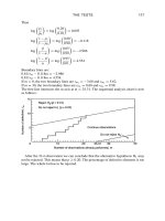
Boundary lines are:
0.811r
m
− 0.118m =−2.986
0.811r
m
− 0.118m = 4.554.
If m = 0, the two boundary lines are r
m
1

=−3.68 and r
m
2
= 5.62.
If m = 30, the two boundary lines are r
m
1
= 0.68 and r
m
2
= 9.98.
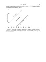
The first line intersects the m-axis at m = 25.31. The sequential analysis chart is now
as follows:
After the 21st observation we can conclude that the alternative hypothesis H
1
may
not be rejected. This means that p
 0.20. The percentage of defective elements is too
large. The whole lot has to be rejected.
GOKA: “CHAP05C” — 2006/6/10 — 17:23 — PAGE 118 — #20
118 100 STATISTICAL TESTS
Test 63 The adjacency test for randomness of
fluctuations
Object
To test the null hypothesis that the fluctuations in a series are random in nature.
Limitations
It is assumed that the observations are obtained independently of each other and under
similar conditions.
Method
For a series of n terms, x

i
(i = 1, , n), the test statistic is defined as
L = 1 −
n−1

i=1
(x
i+1
− x
i
)
2
2
n

i=1
(x
i
−¯x)
2
.
For n > 25, this approximately follows a normal distribution with mean zero and
variance

(n − 2)
(n − 1)(n + 1)
.
For n < 25, critical values for
D =
n−1


i=1
(x
i+1
− x
i
)
2
n

i=1
(x
i
−¯x)
2
are available in Table 28.
In both cases the null hypothesis is rejected if L exceeds the critical values.
Example
An energy forecaster has produced a model of energy demand which she has fitted to
some data for an industry sector over a standard time period. To assess the goodness of
fit of the model she performs a test for randomness on the residuals from the model. If
these are random then the model is a good fit to the data. She calculates the D statistic
and compares it with the values from Table 28 of 1.37 and 2.63. Since D is less then
the lower critical value she rejects the null hypothesis of randomness and concludes
that the model is not a good fit to the data.
GOKA: “CHAP05C” — 2006/6/10 — 17:23 — PAGE 119 — #21
THE TESTS 119
Numerical calculation

x

i
= 2081.94,

x
2
i
= 166 736.9454
n

i=1
(x
i
−¯x)
2
= 26.4006,
n−1

i=1
(x
i+1
− x
i
)
2
= 31.7348, n = 25
D =
n−1

i=1
(x

i+1
− x
i
)
2
n

i=1
(x
i
−¯x)
2
=
31.7348
26.4006
= 1.20
The critical values at α = 0.05 are 1.37 (lower limit) and 2.63 (upper limit) [Table 28].
The calculated value is less than the lower limit.
Hence the null hypothesis is to be rejected.
GOKA: “CHAP05C” — 2006/6/10 — 17:23 — PAGE 120 — #22
120 100 STATISTICAL TESTS
Test 64 The serial correlation test for randomness of
fluctuations
Object
To test the null hypothesis that the fluctuations in a series have a random nature.
Limitations
It is assumed that the observations are obtained independently of each other and under
similar conditions.
Method
The first serial correlation coefficient for a series of n terms, x

i
(i = 1, , n),is
defined as
r
1
=
n
n − 1
⎧
⎪
⎪
⎪
⎪
⎪
⎨
⎪
⎪
⎪
⎪
⎪
⎩
n−1

i=1
(x
i
−¯x)(x
i+1
−¯x)
n


i=1
(x
i
−¯x)
2
⎫
⎪
⎪
⎪
⎪
⎪
⎬
⎪
⎪
⎪
⎪
⎪
⎭
and this forms the test statistic.
For n
 30, critical values for r
1
can be found from Table 29. For n > 30, the normal
distribution provides a reasonable approximation. In both cases the null hypothesis is
rejected if the test statistic exceeds the critical values.
Example
A production line is tested for a systematic trend in the values of a measured charac-
teristic of the components produced. A serial correlation test for randomness is used.
If there is a significant correlation then the quality engineer will look for an assignable

cause and so improve the resulting quality of components. He computes his first serial
correlation as 0.585. The critical value from Table 29 is 0.276. So the correlation
between successive components is significant.
Numerical calculation
x
i
: 69.76, 67.88, 68.28, 68.48, 70.15, 71.25, 69.94, 71.82, 71.27, 68.79, 68.89, 69.70,
69.86, 68.35, 67.61, 67.64, 68.06, 68.72, 69.37, 68.18, 69.35, 69.72, 70.46, 70.94,
69.26, 70.20
n = 26,

x
i
= 1804.38, ¯x = 69.40,

(x
i
−¯x)
2
= 34.169

x
i+1
• x
i
= 125 242.565,

x
i+1
• x

i
−


x
i

2
/n = 19.981
r
1
=
19.981
34.169
= 0.585
The critical value at α = 0.05 is about 0.276 [Table 29].
Hence the null hypothesis is rejected; the correlation between successive observations
is significant.
GOKA: “CHAP05C” — 2006/6/10 — 17:23 — PAGE 121 — #23
THE TESTS 121
Test 65 The turning point test for randomness of
fluctuations
Object
To test the null hypothesis that the variations in a series are independent of the order of
the observations.
Limitations
It is assumed that the number of observations, n, is greater than 15, and the observations
are made under similar conditions.
Method
The number of turning points, i.e. peaks and troughs, in the series is determined and

this value forms the test statistic. For large n, it may be assumed to follow a normal
distribution with mean
2
3
(n−2) and variance (16n−29)/90. If the test statistic exceeds
the critical value, the null hypothesis is rejected.
Example
An investment analyst wishes to examine a time series for a particular investment
portfolio. She is especially keen to know if there are any turning points or if the series
is effectively random in nature. She calculates her test statistic to be 1.31 which is less
than the tabulated value of 1.96 [Table 1]. She concludes that the series is effectively
random and no turning points can be detected.
Numerical calculation
p = peak, t = trough, n = 19, α = 0.05
0.68; 0.34(t); 0.62; 0.73(p); 0.57;
0.32(t); 0.58( p); 0.34(t); 0.59( p); 0.56;
0.49; 0.17(t); 0.30; 0.39; 0.42( p);
0.41(t); 0.46; 0.50; 0.45
Mean =
2
3
× 17 = 11.3, variance =
16 × 19 − 29
90
= 3.05,
standard deviation = 1.75
Test statistic =





9 − 11.3
1.75




= 1.33
The critical value at α = 0.05 is 1.96 [Table 1].
Hence the departure from randomness is not significant.
GOKA: “CHAP05C” — 2006/6/10 — 17:23 — PAGE 122 — #24
122 100 STATISTICAL TESTS
Test 66 The difference sign test for randomness in
a sample
Object
To test the null hypothesis that the fluctuations of a sample are independent of the order
in the sequence.
Limitations
It is assumed that the number of observations is large and that they have been obtained
under similar conditions.
Method
From the sequence of observations a sequence of successive differences is formed. The
number of + signs, p, in this derived sequence forms the test statistic.
Let n be the initial sample size. For large n, p may be assumed to follow a normal
distribution with mean (n − 1)/2 and variance (n + 1)/12. When the test statistic lies
in the critical region the null hypothesis is rejected.
Example
A quality engineer suspects that there is some systematic departure from randomness in
machined component production lines. He uses the difference sign test for randomness
to assess this. His test statistic of 4.54 is for his first sample of size 20 from production

line 1. Since this value is greater than the tabulated value of 1.64 from Table 1 he
concludes that there is a positive trend in this case. In the other samples from the other
production lines he cannot reject the null hypothesis of randomness.
Numerical calculation
n = 20, α = 0.05
List S
1
S
2
S
3
S
4
S
5
p 16 11 10 9 10
Mean =
n − 1
2
=
19
2
= 9.5, variance =
20 +1
12
= 1.75,
standard deviation = 1.32
p(S
1
) =

16 − 9.5 − 0.5
1.32
= 4.54
The critical value at α = 0.05 is 1.64 [Table 1].
Reject the null hypothesis in this case.
However, p(S
2
) = 0.76, p(S
3
) = 0.0, p(S
4
) =−0.76, p(S
5
) = 0.
Do not reject the null hypothesis in these cases, where a positive trend is not indicated.
GOKA: “CHAP05C” — 2006/6/10 — 17:23 — PAGE 123 — #25
THE TESTS 123
Test 67 The run test on successive differences for
randomness in a sample
Object
To test the null hypothesis that observations in a sample are independent of the order
in the sequence.
Limitations
It is necessary that the observations in the sample be obtained under similar conditions.
Method
From the sequence of observations, a sequence of successive differences is formed, i.e.
each observation has the preceding one subtracted from it. The number of runs of +
and − signs in this sequence of differences, K, provides the test statistic.
Let n be the initial sample size. For 5
 n  40, critical values of K can be obtained

from Table 30. For n > 40, K may be assumed to follow a normal distribution with
mean (2n −1)/3 and variance (16n −29)/90. In both cases. when the test statistic lies
in the critical region, the null hypothesis is rejected.
Example
A quality engineer tests five production lines for systematic effects. He uses the run
test on successive differences. He calculates the number of successive plus or minus
signs for each line. He then compares these with the tabulated values of 9 and 17, from
Table 30. For line A his number of runs is 7 which is less than the critical value, 9, so
he rejects the null hypothesis of randomness. The values of 6 and 19 for lines C and
D result in a similar conclusion. The test statistics for lines B and E do not lie in the
critical region so he accepts the null hypothesis for these.
Numerical calculation
Lists A B C D E
Number (K) of runs (plus and minus) 7 12 6 19 12
n = 20, α = 0.05
The critical values are (left) 9 and (right) 17 [Table 30].
For cases A, C and D
K(A) = 7 and K(C) = 6, which are less than 9, and K(D) = 19 which is greater
than 17.
Hence reject the null hypothesis.
For cases B and E
Test statistics do not lie in the critical region [Table 30].
Do not reject the null hypothesis.
GOKA: “CHAP05C” — 2006/6/10 — 17:23 — PAGE 124 — #26
124 100 STATISTICAL TESTS
Test 68 The run test for randomness of two related
samples
Object
To test the null hypothesis that the two samples have been randomly selected from the
same population.

Limitations
It is assumed that the two samples have been taken under similar conditions and that
the observations are independent of each other.
Method
The first sample of n
1
elements are all given a + sign and the second sample of n
2
elements are all given a − sign. The two samples are then merged and arranged in
increasing order of magnitude (the allocated signs are to differentiate between the two
samples and do not affect their magnitudes). A succession of values with the same sign,
i.e. from the same sample, is called a run. The number of runs (K) of the combined
samples is found and is used to calculate the test statistic, Z.Forn
1
and n
2
 10,
Z =
K −µ
K
+
1
2
σ
K
can be compared with the standard normal distribution: here
µ
K
=
2n

1
n
2
n
1
+ n
2
+ 1 and σ
2
K
=
2n
1
n
2
(2n
1
n
2
− n
1
− n
2
)
(n
1
+ n
2
)
2

· (n
1
+ n
2
− 1)
.
When the test statistic lies in the critical region, reject the null hypothesis.
Example
A maintenance programme has been conducted on a plastic forming component produc-
tion line. The supervisor responsible for the line wants to ensure that the maintenance
has not altered the machine settings and so she performs the run test for randomness
of two related samples. She collects two samples from the line, one before the mainte-
nance and one after. The test statistic value is 0.23 which is outside the critical value
of ±1.96. She concludes that the production line is running as usual.
Numerical calculation
n
1
= 10, n
2
= 10, K = 11, α = 0.05
Sample S
1
: 26.3, 28.6, 25.4, 29.2, 27.6, 25.6, 26.4, 27.7, 28.2, 29.0
Sample S
2
: 28.5, 30.0, 28.8. 25.3, 28.4, 26.5, 27.2, 29.3, 26.2, 27.5
GOKA: “CHAP05C” — 2006/6/10 — 17:23 — PAGE 125 — #27
THE TESTS 125
S
1

and S
2
are merged and arranged in increasing order of magnitude, and signs are
allocated to obtain the number of runs K:
−++−++−−−+++−−+−++−−
µ
K
=
2 ×10 ×10
10 +10
+ 1 =
200
20
+ 1 = 11
σ
2
K
=
2 ×10 ×10(2 × 10 × 10 −10 −10)
(10 +10)
2
(10 +10 −1)
= 4.74, σ
K
= 2.18
Z =
11 − 11 +
1
2
2.18

= 0.23. Critical value at α = 0.05 is 1.96 [Table 1].
Hence do not reject the hypothesis.
GOKA: “CHAP05C” — 2006/6/10 — 17:23 — PAGE 126 — #28
126 100 STATISTICAL TESTS
Test 69 The run test for randomness in a sample
Object
To test the significance of the order of the observations in a sample.
Limitations
It is necessary that the observations in the sample be obtained under similar conditions.
Method
All the observations in the sample larger than the median value are given a + sign and
those below the median are given a − sign. If there is an odd number of observations
then the median observation is ignored. This ensures that the number of + signs (n) is
equal to the number of − signs. A succession of values with the same sign is called a
run and the number of runs, K, of the sample in the order of selection is found. This
forms the test statistic.
For n > 30, this test statistic can be compared with a normal distribution with mean
n +1 and variance
1
2
n(2n −2)/(2n −1). The test may be one- or two-tailed depending
on whether we wish to test if K is too high, too low or possibly both.
For n < 30, critical values for K are provided in Table 31. In both cases the null
hypothesis that the observations in the sample occurred in a random order is rejected
if the test statistic lies in the critical region.
Example
A quality control engineer has two similar processes, which produce dual threaded
nuts. He suspects that there is some intermittent fault on atleast one process and so
decides to test for randomness using the run test for randomness. In his first sample,
from process A, he calculates the number of runs of the same sign to be 6. For his

second process, B, he calculates the number of runs to be 11. The critical values are 9
and 19, from Table 31. Since for the process A, 6 is in the critical region, his suspicions
for this process are well founded. Process B shows no departure from randomness.
Numerical calculation
n
1
= n
2
= 13
Sample A
81.02, 80.08, 80.05, 79.70, 79.13, 77.09, 80.09,
(+)(−)(−)(−)(−)(−)(−)
79.40, 80.56, 80.97, 80.17, 81.35, 79.64, 80.82, 81.26,
(−)(+)(+)(+)(+)(−)(+)(+)
80.75, 80.74, 81.59, 80.14, 80.75, 81.01, 79.09,
(+)(+)(+)(+)(+)(+)(−)
78.73, 78.45, 79.56, 79.80
(−)(−)(−)(−)
Median value = 80.12 and number of runs = 6.
GOKA: “CHAP05C” — 2006/6/10 — 17:23 — PAGE 127 — #29
THE TESTS 127
Sample B
69.76, 67.88, 68.28, 68.48, 70.15, 71.25, 69.94,
(+)(−)(−)(−)(+)(+)(+)
71.82, 71.27, 69.70, 68.89, 69.24, 69.86, 68.35,
(+)(+)(+)(−)(−)(+)(−)
67.61, 67.64, 68.06, 68.72, 69.37, 68.18, 69.35,
(−)(−)(−)(−)(+)(−)(−)
69.72, 70.46, 70.94, 69.26, 70.20
(+)(+)(+)(−)(+)

Median value = 69.36 and number of runs = 11.
The critical values at α = 0.10 are (lower) 9 and (upper) 19 [Table 31].
For Sample A number of runs K = 6 lies in the critical region. Hence reject the null
hypothesis (i.e. the fluctuation is not random).
For Sample B number of runs K = 11 does not lie in the critical region.
Do not reject the null hypothesis (i.e. the fluctuation may be considered to be random).
GOKA: “CHAP05C” — 2006/6/10 — 17:23 — PAGE 128 — #30
128 100 STATISTICAL TESTS
Test 70 The Wilcoxon–Mann–Whitney rank sum test
for the randomness of signs
Object
To test that the occurrence of + and − signs in a sequence is random.
Limitations
This is a distribution-free test, applicable if the observations are random and
independent and the two frequency distributions are continuous.
Method
Let n
1
be the number of + or − signs, whichever is the larger, n
2
be the number of
opposite signs and N = n
1
+ n
2
. From the integers describing the natural order of
the signs, the rank sum R of the smallest number of signs is determined. The value
R

= n

2
(N + 1) − R is calculated. The smaller of R and R

is used as the test statistic.
If it is less than the critical value obtained from Table 21 the null hypothesis of random
+ and − signs is rejected.
Example
A simple fuel monitoring system has a target fuel usage level and fuel use is determined
at regular intervals. If the fuel use is higher or lower than the target value then a plus or
minus sign is recorded. Departures from target on either side would signal a potential
problem. An energy monitoring officer has recorded some data and uses the Wilcoxon–
Mann–Witney rank sum test for randomness. He obtains a minimum rank sum of 29
and, since this lies in the critical region (Table 21), he concludes that he has a fuel usage
problem.
Numerical calculation
Successive observations in a sequence are coded with a plus or minus sign:
1234567891011121314
+++−++++−−−+−−
n
1
= 8, n
2
= 6 (minus signs), N = 14
Rank sum of minus signs = 4 + 9 + 10 +11 +13 +14 = 61
R

= 6(14 + 1) − 61 = 29
The critical value at α = 0.025 is 29 [Table 21].
Reject the null hypothesis; alternatively, the experiment could be repeated.
GOKA: “CHAP05C” — 2006/6/10 — 17:23 — PAGE 129 — #31

THE TESTS 129
Test 71 The rank correlation test for randomness of
a sample
Object
To test that the fluctuations in a sample have a random nature. This test may be used to
test the elements of a time series for the presence of a trend.
Limitations
This is a distribution-free test, applicable if the observations occur in a natural sequence
and have been obtained under similar or comparable conditions. It is sensitive to the
occurrence of a positive or negative trend, and relatively insensitive to the occurrence
of sudden jumps.
Method
The observations are ranked in increasing order of magnitude R
i
. The correlation
between these rank and the integers representing the natural order of the observations
is then calculated. This can be tested using the Spearman rank correlation test (Test 58)
or the Kendall rank correlation test (Test 59). If the sample is larger than the T statistic
T can be compared with the critical value of the normal distribution.
Example
A merchandising manager observes the sales of a particular item of clothing across all
her stores. She is looking for a discernable trend so that she can be pre-emptive of stock
challenges. She produces a Spearman rank correlation between the natural order and
the sorted data order of 0.771. Her T statistic is 3.36 which is in the critical region. She
thus rejects the null hypothesis of randomness and is able to adjust production levels
to account for this trend.
Numerical calculation
Order (x
i
)12345678910

Obs. 98 101 110 105 99 106 104 109 100 102
Rank (y
i
) 14107286935
Order (x
i
) 11 12 13 14 15 16 17 18 19 20
Obs. 119 123 118 116 122 130 115 124 127 114
Rank (y
i
) 15 17 14 13 16 20 12 18 19 11

(x
i
− y
i
)
2
= 304 = R
r
R
= 1 −
6R
n(n
2
− 1)
= 0.771
T =
6R − n(n
2

− 1)
n(n + 1)
√
n − 1
=−3.36
The critical value at α = 0.05 is 1.96 [Table 1].
The calculated value is greater than the critical value.
Reject the null hypothesis.
GOKA: “CHAP05C” — 2006/6/10 — 17:23 — PAGE 130 — #32
130 100 STATISTICAL TESTS
Test 72 The Wilcoxon–Wilcox test for comparison of
multiple treatments of a series of subjects
Object
To compare the significance of the difference in response for K treatments applied to n
subjects.
Limitations
It is assumed that a subject’s response to one treatment is not affected by the same
subject’s response to another treatment; and that the response distribution for each
subject is continuous.
Method
The data are represented by a table of n rows and K columns. The rank numbers
1, 2, , K are assigned to each row and then the sum of the rank numbers for each
column, R
j
( j = 1, 2, , K) is determined. A pair of treatments, say p and q, can
now be compared by using as test statistic |R
p
− R
q
|. If this exceeds the critical value

obtained from Table 32 the null hypothesis of equal effects of the p and q treatments is
rejected.
Example
Six different ice cream flavours are compared by six tasters who assign a score (1 to 25)
to each flavour. The food technologist wishes to compare each flavour with the others
and uses the Wilcoxon–Wilcox test of multiple treatments. She finds that the rank sum
difference for the flavours comparisons A–E, A–F and D–F are significant.
Numerical calculation
Rank sums
Sample
Serial no. A B C D E F
1 153246
2 136245
3 234156
4 143265
5 253146
6 136245
Rank sum 8 23 25 10 27 33
Rank sum differences |R
p
− Rq|
DBC E F
A8 2 15 17 19* 25*
D10
13 15 17 23*
B23
24 10
C25
28
E27

6
* Exceeds critical value.
K = 6, n = 6, α = 0.05, critical value = 18.5 [Table 32].
GOKA: “CHAP05C” — 2006/6/10 — 17:23 — PAGE 131 — #33
THE TESTS 131
Test 73 Friedman’s test for multiple treatment of
a series of subjects
Object
To investigate the significance of the differences in response for K treatments applied
to n subjects.
Limitations
It is assumed that a subject’s response to one treatment is not affected by the same
subject’s response to another treatment; and that the response distribution for each
subject is continuous.
Method
The data can be represented by a table of n rows and K columns. In each row the
rank numbers 1, 2, , K are assigned in order of increasing value. For each of the K
columns the rank sum R
j
( j = 1, 2, , K) is determined.
The test statistic is
G =
12
nK(K + 1)
K

j=1
R
2
j

− 3n(K + 1).
If this exceeds the critical χ
2
value obtained from Table 5 with K −1 degrees of freedom,
the null hypothesis that the effects of the K treatments are all the same is rejected.
If ties occur in the ranking procedure one has to assign the average rank member for
each series of equal results. In this case the test statistic becomes
G =
12(K − 1)S
nK
3
− D
where S =

K
j=1
(R
j
−
¯
R)
2
and D =

f
i
t
3
i
.

Example
Four different newspaper advertisement styles are compared to see if they produce
the same effect on a panel of viewers/consumers. The different styles relate to size
and position. There are 15 panel members and they rank each advertisement. The test
statistic produced by this procedure is 12.51. The critical value from Table 5 is 7.81.
So we conclude that the advertisement styles are not equally effective.
Numerical calculation
t
i
is the size of the ith group of equal observations.
n = 15, K = 4,
¯
R =
n(K + 1)
2
GOKA: “CHAP05C” — 2006/6/10 — 17:23 — PAGE 132 — #34
132 100 STATISTICAL TESTS
Rank numbers (showing many ties)
Columns (K)
Rows (n) c
1
c
2
c
3
c
4
1 3.5 3.5 1.5 1.5
2 4.0 2.0 2.0 2.0
3 1.5 3.5 2.5 2.5

4 3.5 3.5 1.5 1.5
5 3.0 3.0 3.0 1.0
6 3.0 3.0 1.0 3.0
7 3.5 1.5 3.5 1.5
8 2.5 2.5 2.5 2.5
9 3.0 3.0 1.0 3.0
10 2.5 2.5 2.5 2.5
11 3.5 1.5 3.5 1.5
12 4.0 2.0 2.0 2.0
13 2.5 2.5 2.5 2.5
14 3.0 3.0 3.0 1.0
15 4.0 2.0 3.0 1.0
R
j
47 39 35 29
¯
R 37.5 37.5 37.5 37.5
R
j
−
¯
R +9.5 +1.5 −2.5 −8.5
S =

(R
j
−
¯
R)
2

= 171
Here 1, 2, 3 and 4 are the size of the groups of equal observations and D =

f
i
t
3
i
.
t
i
f
i
f
i
t
i
f
i
t
3
i
1777
2102080
3 7 21 189
4 3 12 192
Total 60 468
Hence D = 468
G =
12 ×(4 −1) ×171

15 × 4
3
− 468
= 12.51
The critical value is χ
2
3;005
= 7.81 [Table 5].
Since G > 7.81, reject the null hypothesis.
GOKA: “CHAP05C” — 2006/6/10 — 17:23 — PAGE 133 — #35
THE TESTS 133
Test 74 The rank correlation test for agreement in
multiple judgements
Object
To investigate the significance of the correlation between n series of rank numbers,
assigned by n members of a committee to K subjects.
Limitations
This test can be applied if the judges decide independently and if the subjects show
obvious differences in the quality being judged.
Method
Let n judges give rank numbers to K subjects.
Compute S = nK(K
2
− 1)/12 and S
D
= the sum of squares of the differences
between subjects’ mean ranks and the overall mean rank. Let
D
1
=

S
D
n
1
, D
2
= S −D
1
, S
2
1
=
D
1
K −1
, S
2
2
=
D
2
K(n − 1)
.
The test statistic is F = S
2
1
/S
2
2
which follows the F-distribution with (K −1, K(n −1))

degrees of freedom. If this exceeds the critical value obtained from Table 3, the null
hypothesis of agreement between the judgements is rejected.
Example
A wine tasting panel is selected by asking a number of questions and also by tasting
assessment. In one assessment three judges are compared for agreement. One of the
judges is an expert taster. Ten wines are taken and the judges are asked to rank them
on a particular taste criterion. Are the three judges consistent? The test statistic, F is
0.60,which is less than the tabulated value of 2.39. So the new panel members can be
recruited.
Numerical calculation
n = 3, K = 10, ν
1
= K −1 = 9, ν
2
= K(n − 1) = 20
Rank number
A B C D E F G H I J Total
Judge 1 1 2 3 4 567891055
Judge 2 7 10 4 168952355
Judge 3 9 6 10 3 5 4 7 8 2 1 55
Total score 17 18 17 8 16 18 23 21 13 14 165
Mean 16.5 16.5 16.5 16.5 16.5 16.5 16.5 16.5 16.5 16.5 165
Difference 0.5 1.5 0.5 −8.5 −0.5 1.5 6.5 4.5 −3.5 −2.5
GOKA: “CHAP05C” — 2006/6/10 — 17:23 — PAGE 134 — #36
134 100 STATISTICAL TESTS
S =
3 × 10(100 −1)
12
= 247.5, S
D

= 158.50,
D
1
=
158.50
3
= 52.83, D
2
= S −D
1
= 247.50 −52.83 = 194.67,
S
2
1
=
52.83
9
= 5.87, S
2
2
=
194.67
10 ×2
=
194.67
20
= 9.73
F = S
2
1

/S
2
2
=
5.87
9.73
= 0.60
Critical value F
9; 20; 0.05
= 2.39 [Table 3].
Do not reject the null hypothesis.
GOKA: “CHAP05C” — 2006/6/10 — 17:23 — PAGE 135 — #37
THE TESTS 135
Test 75 A test for the continuous distribution of
a random variable
Object
To test a model for the distribution of a random variable of the continuous type.
Limitations
This test is applicable if some known continuous distribution function is being tested.
A partition of the random values into different sets must be available using the closed
interval [0.1].
Method
Let F(W) be the distribution function of W which we want to test. The null hypothesis
is
H
0
: F(W) = F
0
(W)
where F

0
(W) is some known continuous distribution function.
The test is based on the χ
2
statistic. In order to use this, we must partition the set
of possible values of W into k (not necessarily equal) sets. Partition the interval [0, 1]
into k sets such that 0 = b
0
< ···< b
k
= 1. Let a
i
= F
−1
0
(b
i
), i = 1, 2, , k − 1,
A
1
=[−α, a
1
], A
i
=[−a
i−1
, a
i
], for i = 2, 3, , k − 1 and A
k

= (a
k−1
, α); p
i
=
P (W ∈ A
i
), i = 1, 2, , k. Let Y
i
denote the number of times the observed value of
W belongs to A
i
, i = 1, 2, , k in n independent repetitions of the experiment. Then
Y
1
, Y
2
, , Y
k
have a multinomial distribution with parameters n, p
1
, p
2
, , p
k
. Let
π
i
= P (W ∈ A
i

) when the distribution function of W is F
0
(W).
Then we test the hypothesis:
H
∗
0
: p
i
= π
i
, i = 1, 2, , k.
H
∗
0
is rejected if the observed value of the χ
2
statistic
Q
k−1
=
k−1

i=1
(Y
i
− nπ
i
)
2

nπ
i
is at least as great as C, where C is selected to yield the desired significance level.
Example
A continuous distribution is tested by calculating Q
9
which follows approximately a
chi-squared distribution. The value of 4.0 is compared with 16.92 from Table 5. Since
the calculated value is not in the critical region, the null hypothesis that the data follows
the given continuous distribution is accepted.
GOKA: “CHAP05C” — 2006/6/10 — 17:23 — PAGE 136 — #38
136 100 STATISTICAL TESTS
Numerical calculation
Let W denote the outcome of a random experiment. Let F(W) denote the distribution
function of W and let
F
0
(W) =
⎧
⎪
⎨
⎪
⎩
0, W < −1
1
2
(W
3
+ 1), −1  W < 1
1, W

 1.
The interval [−1, 1] can be partitioned into 10 sets of equal probability with the point
b
i
= i/10, i = 0, 1, ,10.
If a
i
= F
−1
(b
i
) = (2b
i
− 1)
1
3
, i = 1, 2, , 9 then the sets A
1
=[−1, a
1
], A
2
=
[a
1
, a
2
], , A
10
=[A

9
,1]will each have probability 0.1. If the random sample of size
n = 50 is observed then nπ
i
= 50 × 0.1 = 5.0. Let the summary of the 50 observed
values be
A
1
= 6, A
2
= 4, A
3
= 5, A
4
= 6, A
5
= 4, A
6
= 4, A
7
= 6, A
8
= 8, A
9
= 3, A
10
= 4.
Then the calculated value of Q
9
is

Q
9
=
(6 − 5)
2
5
+
(4 − 5)
2
5
+···+
(4 − 5)
2
5
= 4.0.
Critical value χ
2
9;0.05
= 16.92 [Table 5].
Hence do not reject the null hypothesis.
GOKA: “CHAP05D” — 2006/6/10 — 17:23 — PAGE 137 — #1
THE TESTS 137
Test 76 A test for the equality of multinomial
distributions
Object
To test the equality of h independent multinomial distributions.
Limitations
If p
i
is the probability of an item being assigned to the i th class, then this test is applicable

if y
ij
is the number of items occurring in the class associated with p
i
.
Method
Let p
ij
= P (A
i
), i = 1, 2, , k; j = 1, 2, , h. It is required to test
H
0
: p
i1
= p
i2
=···=p
ih
= p
i
, i = 1, 2, , k.
Carry out the jth experiment n
j
times, making sure that the n
j
instances are independent,
and let Y
1j
, Y

2j
, , Y
kj
denote the frequencies of the respective events A
1
, A
2
, , A
k
.
Then
Q =
h

j=1
k

i=1
(Y
ij
− n
j
p
ij
)
2
n
j
p
ij

has an approximate χ
2
-distribution with h(k − 1) degrees of freedom. Under H
0
we
estimate k − 1 probabilities from
ˆp
i
=
h

j=1
Y
ij
h

j=1
n
j
, i = 1, 2, , k −1;
the estimate of p
k
then follows from ˆp
k
= 1 −

k−1
i=1
ˆp
i

. Then
Q =
h

j=1
k

i=1
(Y
ij
− n
j
ˆp
i
)
2
n
j
ˆp
i
has an approximate χ
2
-distribution with
h(k − 1) − (k − 1) = (h − 1)(k − 1)
degrees of freedom.
GOKA: “CHAP05D” — 2006/6/10 — 17:23 — PAGE 138 — #2
138 100 STATISTICAL TESTS
Example
An electronic allocation of visual stimuli to one of five categories, or grades ensures
that the allocations are equally likely and not subject to any bias effects. An experiment

to allocate 50 stimuli to 5 grades is repeated once. Are the allocations equally likely?
The computed Q statistic of 5.18 is less than the tabulated value of 9.488 (Table 5) so
there is no justification to suspect unequal allocation probabilities.
Numerical calculation
Grade
Group A
1
A
2
A
3
A
4
A
5
Total
1 8 13 16 10 3 50
2491416750
n = 50
P (A
1
) =
8 + 4
100
= 0.12, P(A
2
) = 0.22, P(A
3
) = 0.30
P (A

4
) = 0.26, P(A
5
) = 0.10
Thus we have estimates of n
1
P
i1
= 6, n
2
P
i2
= 11, n
3
P
i3
= 15, n
4
P
i4
= 13 and
n
5
P
i5
= 5, respectively.
Hence the computed value of Q is:
Q =
(8 − 6)
2

6
+
(13 − 11)
2
11
+
(16 − 15)
2
15
+
(10 −13)
2
13
+
(3 − 5)
2
5
+
(4 − 6)
2
6
+
(9 − 11)
2
11
+
(14 − 15)
2
15
+

(16 − 13)
2
13
+
(7 − 5)
2
5
= 5.18
The critical value is χ
2
4; 005
= 9.488 [Table 5].
The calculated value is less than the critical value. Do not reject the null hypothesis.
GOKA: “CHAP05D” — 2006/6/10 — 17:23 — PAGE 139 — #3
THE TESTS 139
Test 77 F -test for non-additivity
Object
To test for non-additivity in a two-way classification.
Limitations
This test is applicable if the observations are independently and normally distributed
with constant variance.
Method
In the two-way classification with one observation per cell (fixed effects model), we
assume additivity (absence of interaction effects). In the case of any doubt about this
additivity, Tukey proposed a test under the following set-up:
Y
ij
= µ + α
i
+ β

j
+ λα
i
β
j
+ e
ij
subject to the conditions that

i
α
i
=

j
β
j
= 0
and that the e
ij
are independently N(0, σ
2
). Under this set-up, the interaction effect is
represented by λα
i
β
j
, where

i

all j
λα
i
β
j
=

j
all i
λα
i
β
j
= 0.
A test for non-additivity is obtained by a test for H
0
: λ = 0 or equivalently by a test
H
0
: E(Y
ij
) = µ + α
i
+ β
j
under this set-up. But this set-up does not conform to the
Gauss–Markov model for E(Y
ij
) which are not linear in the parameter µ, α
i

, β
j
and λ.
A set of unbiased estimators for, µ, α
i
and β
j
are:
µ
∗
= Y
00
, α
∗
i
= Y
i0
− Y
00
, β
∗
j
= Y
0j
− Y
00
.
The least squares (unbiased) estimator of λ is obtained by minimizing
s
2

E
=

i

j
(Y
ij
− µ − α
i
− β
j
− λα
i
β
j
)
2
with respect to λ under the assumption that α
i
and β
j
are known. Thus
λ
∗
=

i

j

α
i
β
j
Y
ij

i
α
2
i

j
β
2
j
.
GOKA: “CHAP05D” — 2006/6/10 — 17:23 — PAGE 140 — #4
140 100 STATISTICAL TESTS
Then the sum of squares due to interaction, i.e. due to λ
∗
,isgivenby
s
2
λ
∗
=
⎡
⎣


i

j
α
i
β
j
Y
ij
⎤
⎦
2

i
α
2
i

j
β
2
j
with l degrees of freedom. The sum of squares due to non-additivity is given by
s
2
N
=
⎡
⎣


i

j
α
∗
i
β
∗
j
Y
ij
⎤
⎦
2

i
α
∗2
i

j
β
∗2
j
.
For all given α
∗
i
, β
∗

j
, for all i, j, we have that s
2
N
/σ
2
and (s
2
E
− s
2
N
)/σ
2
= s
2
R
are
independent and have χ
2
-distribution with 1 and ( p−1)(q−1)−1 degrees of freedom,
respectively.
We reject H
0
: λ = 0atlevelα if the variance ratio for non-additivity is too large,
i.e. if
[( p − 1)(q − 1) − 1]
s
2
N

s
2
R
> F
1,(p−1)(q−1)−1; α
and fail to reject otherwise.
Example
A thermal bond is tested to assess whether the resultant strength of the bond is the result
of the combination of the main effects of temperature and pressure only. That is, no
temperature/pressure interaction exists. There are four levels of temperature and three
levels of pressure. The F test statistic for non-additivity is 0.2236 which is compared
with the critical tabulated value of 6.61 [Table 3]. Since the calculated F is less than
the critical value the assumption of no interaction is upheld.
Numerical calculation
j
i 123 4 Y
i0
¯
Y
i0
1
14 2 1 2 19 4.75
2 202 2 61.5
3 215 0 82
Y
0j
1838 4 33
¯
Y
0j

6 1 2.7 1.33
GOKA: “CHAP05D” — 2006/6/10 — 17:23 — PAGE 141 — #5
THE TESTS 141
µ = Y
00
=
33
12
= 2.75
α
∗
1
= 19 − 2.75 = 16.25, α
∗
2
= 3.25, α
∗
3
= 5.25
β
∗
1
= 18 − 2.75 = 15.25, β
∗
2
= 0.25, β
∗
3
= 5.25, β
∗

4
= 1.25
λ
∗
=
4023.75
79 229.788
= 0.05079, s
2
E
= 4568.38, s
2
N
= 204.35
Let σ
2
= 16, then
s
2
E
σ
2
= 285.52 and
s
2
N
σ
2
= 12.77, s
2

R
= 272.75.
Hence F =
12.77/1
285.52/5
= 0.2236.
Critical value F
1.5; 0.52
= 6.61 [Table 3].
We do not reject the null hypothesis λ = 0.