We set a = e
C
and obtain
L


∞
0
x
ν
e
–Cν
Γ(ν +1)
dν

=
1
p (ln p + C)
. (12)
Let us proceed with relation (9). By (12), we have
f

x
(0)
p (ln p + C)
= L

f

x
(0)


∞
0
x
ν
e
–Cν
Γ(ν +1)
dν

. (13)
Taking into account (10) and (12), we can regard the first summand on the right-hand side in (9) as
a product of transforms. To find this summand itself we apply the convolution theorem:
p
2
˜
f(p) – f

x
(0)
p (ln p + C)
= L


x
0
f

tt
(t)


∞
0
(x – t)
ν
e
–Cν
Γ(ν +1)
dν dt

. (14)
On the basis of relations (9), (13), and (14) we obtain the solution of the integral equation (4) in
the form
y(x)=–

x
0
f

tt
(t)

∞
0
(x – t)
ν
e
–Cν
Γ(ν +1)
dν dt – f


x
(0)

∞
0
x
ν
e
–Cν
Γ(ν +1)
dν. (15)
•
References for Section 8.6: V. Volterra (1959), M. L. Krasnov, A. I. Kiselev, and G. I. Makarenko (1971).
8.7. Method of Quadratures
8.7-1. Quadrature Formulas
The method of quadratures is a method for constructing an approximate solution of an integral
equation based on the replacement of integrals by finite sums according to some formula. Such
formulas are called quadrature formulas and, in general, have the form

b
a
ψ(x) dx =
n

i=1
A
i
ψ(x
i

)+ε
n
[ψ], (1)
where x
i
(i =1, , n) are the abscissas of the partition points of the integration interval [a, b], or
quadrature (interpolation) nodes, A
i
(i =1, , n) are numerical coefficients independent of the
choice of the function ψ(x), and ε
n
[ψ] is the remainder (the truncation error) of formula (1). As a
rule, A
i
≥ 0 and
n

i=1
A
i
= b – a.
There are quite a few quadrature formulas of the form (1). The following formulas are the
simplest and most frequently used in practice.
Rectangle rule:
A
1
= A
2
= ···= A
n–1

= h, A
n
=0,
h =
b – a
n – 1
, x
i
= a + h(i – 1) (i =1, , n).
(2)
Trapezoidal rule:
A
1
= A
n
=
1
2
h, A
2
= A
3
= ···= A
n–1
= h,
h =
b – a
n – 1
, x
i

= a + h(i – 1) (i =1, , n).
(3)
Simpson’s rule (or prizmoidal formula):
A
1
= A
2m+1
=
1
3
h, A
2
= ···= A
2m
=
4
3
h, A
3
= ···= A
2m–1
=
2
3
h,
h =
b – a
n – 1
, x
i

= a + h(i – 1) (n =2m +1, i =1, , n),
(4)
where m is a positive integer.
In formulas (2)–(4), h is a constant integration step.
The quadrature formulas due to Chebyshev and Gauss with various numbers of interpolation
nodes are also widely applied. Let us illustrate these formulas by an example.
Page 454
© 1998 by CRC Press LLC
© 1998 by CRC Press LLC
Example. For the interval [–1, 1], the parameters in formula (1) acquire the following values:
Chebyshev’s formula (n = 6):
A
1
= A
2
= ···=
2
n
=
1
3
,
x
2
= –x
5
= –0.4225186538,
x
1
= –x

6
= –0.8662468181,
x
3
= –x
4
= –0.2666354015.
(5)
Gauss’ formula (n = 7):
A
1
= A
7
= 0.1294849662,
A
3
= A
5
= 0.3818300505,
x
1
= –x
7
= –0.9491079123,
x
3
= –x
5
= –0.4058451514,
A

2
= A
6
= 0.2797053915,
A
4
= 0.4179591837,
x
2
= –x
6
= –0.7415311856,
x
4
=0.
(6)
Note that a vast literature is devoted to quadrature formulas, and the reader can find books of
interest (e.g., see G. A. Korn and T. M. Korn (1968), N. S. Bakhvalov (1973), S. M. Nikol’skii
(1979)).
8.7-2. The General Scheme of the Method
Let us solve the Volterra integral equation of the first kind

x
a
K(x, t)y(t) dt = f(x), f(a)=0, (7)
on an interval a ≤ x ≤ b by the method of quadratures. The procedure of constructing the solution
involves two stages:
1
◦
. First, we determine the initial value y(a). To this end, we differentiate Eq. (7) with respect to x,

thus obtaining
K(x, x)y(x)+

x
a
K

x
(x, t)y(t) dt = f

x
(x).
By setting x = a,wefind that
y
1
= y(a)=
f

x
(a)
K(a, a)
=
f

x
(a)
K
11
.
2

◦
. Let us choose a constant integration step h and consider the discrete set of points x
i
= a+h(i–1),
i =1, , n.Forx = x
i
, Eq. (7) acquires the form

x
i
a
K(x
i
, t)y(t) dt = f(x
i
), i =2, , n, (8)
Applying the quadrature formula (1) to the integral in (8) and choosing x
j
(j =1, , i)tobethe
nodes in t, we arrive at the system of equations
i

j=1
A
ij
K(x
i
, x
j
)y(x

j
)=f(x
i
)+ε
i
[y], i =2, , n, (9)
where the A
ij
are the coefficients of the quadrature formula on the interval [a, x
i
] and ε
i
[y]isthe
truncation error. Assume that the ε
i
[y] are small and neglect them; then we obtain a system of linear
algebraic equations in the form
i

j=1
A
ij
K
ij
y
j
= f
i
, i =2, , n, (10)
Page 455

© 1998 by CRC Press LLC
© 1998 by CRC Press LLC
where K
ij
= K(x
i
, x
j
)(j =1, , i), f
i
= f (x
i
), and y
j
are approximate values of the unknown
function at the nodes x
i
.
Now system (10) permits one, provided that A
ii
K
ii
≠ 0(i =2, , n), to successively find the
desired approximate values by the formulas
y
1
=
f

x

(a)
K
11
, y
2
=
f
2
– A
21
K
21
y
1
A
22
K
22
, , y
n
=
f
n
–
n–1

j=1
A
nj
K

nj
y
j
A
nn
K
nn
,
whose specific form depends on the choice of the quadrature formula.
8.7-3. An Algorithm Based on the Trapezoidal Rule
According to the trapezoidal rule (3), we have
A
i1
= A
ii
=
1
2
h, A
i2
= ···= A
i,i–1
= h, i =2, , n.
The application of the trapezoidal rule in the general scheme leads to the following step algorithm:
y
1
=
f

x

(a)
K
11
, f

x
(a)=
–3f
1
+4f
2
– f
3
2h
,
y
i
=
2
K
ii

f
i
h
–
i–1

j=1
β

j
K
ij
y
j

, β
j
=

1
2
for j =1,
1 for j >1,
i =2, , n,
where the notation coincides with that introduced in Subsection 8.7-2. The trapezoidal rule is quite
simple and effective and frequently used in practice for solving integral equations with variable limit
of integration.
On the basis of Subsections 8.7-1 and 8.7-2, one can write out similar expressions for other
quadrature formulas. However, they must be used with care. For example, the application of
Simpson’s rule must be alternated, for odd nodes, with some other rule, e.g., the rectangle rule or
the trapezoidal rule. For equations with variable integration limit, the use of Chebyshev’s formula
or Gauss’ formula also has some difficulties as well.
8.7-4. An Algorithm for an Equation With Degenerate Kernel
A general property of the algorithms of the method of quadratures in the solution of the Volterra
equations of the first kind with arbitrary kernel is that the amount of computational work at each
step is proportional to the number of the step: all operations of the previous step are repeated with
new data and another term in the sum is added.
However, if the kernel in Eq. (7) is degenerate, i.e.,
K(x, t)=

m

k=1
p
k
(x)q
k
(t), (11)
or if the kernel under consideration can be approximated by a degenerate kernel, then an algorithm can
be constructed for which the number of operations does not depend on the index of the digitalization
node. With regard to (11), Eq. (7) becomes
m

k=1
p
k
(x)

x
a
q
k
(t)y(t) dt = f(x). (12)
Page 456
© 1998 by CRC Press LLC
© 1998 by CRC Press LLC
By applying the trapezoidal rule to (12), we obtain recurrent expressions for the solution of the
equation (see formulas in Subsection 8.7-3):
y(a)=
f


x
(a)
m

k=1
p
k
(a)q
k
(a)
, y
i
=
2
m

k=1
p
ki
q
ki

f
i
h
–
m

k=1

p
ki
i–1

j=1
β
j
q
kj
y
j

,
where y
i
are approximate values of y(x)atx
i
, f
i
= f(x
i
), p
ki
= p
k
(x
i
), and q
ki
= q

k
(x
i
).
•
References for Section 8.7: G. A. Korn and T. M. Korn (1968), N. S. Bakhvalov (1973), V. I. Krylov, V. V. Bobkov, and
P. I. Monastyrnyi (1984), A. F. Verlan’ and V. S. Sizikov (1986).
8.8. Equations With Infinite Integration Limit
Integral equations of the first kind with difference kernel in which one of the limits of integration
is variable and the other is infinite are of interest. Sometimes the kernels and the functions of these
equations do not belong to the classes described in the beginning of the chapter. The investigation
of these equations can be performed by the method of model solutions (see Section 9.6) or by the
method of reducing to equations of the convolution type. Let us consider these methods for an
example of an equation of the first kind with variable lower limit of integration.
8.8-1. An Equation of the First Kind With Variable Lower Limit of Integration
Consider the equation of the first kind with difference kernel

∞
x
K(x – t)y(t) dt = f(x). (1)
Equation (1) cannot be solved by direct application of the Laplace transform, because the convolution
theorem cannot be used here. According to the method of model solutions whose detailed exposition
can be found in Section 9.6, we consider the auxiliary equation with exponential right-hand side

∞
x
K(x – t)y(t) dt = e
px
. (2)
The solution of (2) has the form

Y (x, p)=
1
˜
K(–p)
e
px
,
˜
K(–p)=

∞
0
K(–z)e
pz
dz. (3)
On the basis of these formulas and formula (11) from Section 9.6, we obtain the solution of Eq. (1)
for an arbitrary right-hand side f(x) in the form
y(x)=
1
2πi

c+i∞
c–i∞
˜
f(p)
˜
K(–p)
e
px
dp, (4)

where
˜
f(p) is the Laplace transform of the function f(x).
Page 457
© 1998 by CRC Press LLC
© 1998 by CRC Press LLC
Example. Consider the following integral equation of the first kind with variable lower limit of integration:

∞
x
e
a(x–t)
y(t) dt = A sin(bx), a >0. (5)
According to (3) and (4), we can write out the expressions for
˜
f(p) (see Supplement 4) and
˜
K(–p),
˜
f(p)=
Ab
p
2
+ b
2
,
˜
K(–p)=

∞

0
e
(p–a)z
dz =
1
a – p
,
(6)
and the solution of Eq. (5) in the form
y(x)=
1
2πi

c+i∞
c–i∞
Ab(a – p)
p
2
+ b
2
e
px
dp. (7)
Now using the tables of inverse Laplace transforms (see Supplement 5), we obtain the exact solution
y(x)=Aa sin(bx) – Ab cos(bx), a >0,
(8)
which can readily be verified by substituting (8) into (5) and using the tables of integrals in Supplement 2.
8.8-2. Reduction to a Wiener–Hopf Equation of the First Kind
Equation (1) can be reduced to a first-kind one-sided equation


∞
0
K
–
(x – t)y(t) dt = –f(x), 0 < x < ∞, (9)
where the kernel K
–
(x – t) has the following form:
K
–
(s)=

0 for s >0,
–K(s) for s <0.
Methods for studying Eq. (9) are described in Chapter 10.
•
References for Section 8.8: F. D. Gakhov and Yu. I. Cherskii (1978), A. D. Polyanin and A. V. Manzhirov (1997).
Page 458
© 1998 by CRC Press LLC
© 1998 by CRC Press LLC
Chapter 9
Methods for Solving Linear Equations
of the Form
y(x)–

x
a
K(x, t)y(t) dt = f(x)
9.1. Volterra Integral Equations of the Second Kind
9.1-1. Preliminary Remarks. Equations for the Resolvent

In this chapter we present methods for solving Volterra integral equations of the second kind, which
have the form
y(x)–

x
a
K(x, t)y(t) dt = f(x), (1)
where y(x) is the unknown function (a ≤ x ≤ b), K(x, t) is the kernel of the integral equation, and
f(x) is the right-hand side of the integral equation. The function classes to which y(x), f(x), and
K(x, t) can belong are defined in Subsection 8.1-1. In these function classes, there exists a unique
solution of the Volterra integral equation of the second kind.
Equation (1) is said to be homogeneous if f(x) ≡ 0 and nonhomogeneous otherwise.
The kernel K(x, t) is said to be degenerate if it can be represented in the form K(x, t)=
g
1
(x)h
1
(t)+···+ g
n
(x)h
n
(t).
The kernel K(x, t) of an integral equation is called difference kernel if it depends only on the
difference of the arguments, K(x, t)=K(x – t).
Remark 1. A homogeneous Volterra integral equation of the second kind has only the trivial
solution.
Remark 2. The existence and uniqueness of the solution of a Volterra integral equation of the
second kind hold for a much wider class of kernels and functions.
Remark 3. A Volterra equation of the second kind can be regarded as a Fredholm equation of
the second kind whose kernel K(x, t) vanishes for t > x (see Chapter 11).

Remark 4. The case in which a =–∞ and/or b = ∞ is not excluded, but in this case the square
integrability of the kernel K(x, t) on the square S = {a ≤ x ≤ b, a ≤ t ≤ b} is especially significant.
The solution of Eq. (1) can be presented in the form
y(x)=f(x)+

x
a
R(x, t)f(t) dt, (2)
where the resolvent R(x, t) is independent of f (x) and the lower limit of integration a and is
determined by the kernel of the integral equation alone.
The resolvent of the Volterra equation (1) satisfies the following two integral equations:
R(x, t)=K(x, t)+

x
t
K(x, s)R(s, t) ds , (3)
Page 459
© 1998 by CRC Press LLC
© 1998 by CRC Press LLC
R(x, t)=K(x, t)+

x
t
K(s, t)R(x, s) ds , (4)
in which the integration is performed with respect to different pairs of variables of the kernel and
the resolvent.
9.1-2. A Relationship Between Solutions of Some Integral Equations
Let us present two useful formulas that express the solution of one integral equation via the solutions
of other integral equations.
1

◦
. Assume that the Volterra equation of the second kind with kernel K(x, t) has a resolvent R(x, t).
Then the Volterra equation of the second kind with kernel K
∗
(x, t)=–K(t, x) has the resolvent
R
∗
(x, t)=–R(t, x).
2
◦
. Assume that two Volterra equations of the second kind with kernels K
1
(x, t) and K
2
(x, t) are
given and that resolvents R
1
(x, t) and R
2
(x, t) correspond to these equations. In this case the Volterra
equation with kernel
K(x, t)=K
1
(x, t)+K
2
(x, t) –

x
t
K

1
(x, s)K
2
(s, t) ds (5)
has the resolvent
R(x, t)=R
1
(x, t)+R
2
(x, t)+

x
t
R
1
(s, t)R
2
(x, s) ds. (6)
Note that in formulas (5) and (6), the integration is performed with respect to different pairs of
variables.
•
References for Section 9.1: E. Goursat (1923), H. M. M
¨
untz (1934), V. Volterra (1959), S. G. Mikhlin (1960),
M. L. Krasnov, A. I. Kiselev, and G. I. Makarenko (1971), J. A. Cochran (1972), V. I. Smirnov (1974), P. P. Zabreyko,
A. I. Koshelev, et al. (1975), A. J. Jerry (1985), F. G. Tricomi (1985), A. F. Verlan’ and V. S. Sizikov (1986), G. Gripenberg,
S O. Londen, and O. Staffans (1990), C. Corduneanu (1991), R. Gorenflo and S. Vessella (1991), A. C. Pipkin (1991).
9.2. Equations With Degenerate Kernel:
K(x, t)=g
1

(x)h
1
(t)+···+ g
n
(x)h
n
(t)
9.2-1. Equations With Kernel of the Form K(x, t)=ϕ(x)+ψ(x)(x – t)
The solution of a Volterra equation (see Subsection 9.1-1) with kernel of this type can be expressed
by the formula
y = w

xx
, (1)
where w = w(x) is the solution of the second-order linear nonhomogeneous ordinary differential
equation
w

xx
– ϕ(x)w

x
– ψ(x)w = f (x), (2)
with the initial conditions
w(a)=w

x
(a) = 0. (3)
Let w
1

= w
1
(x) be a nontrivial particular solution of the corresponding homogeneous linear differ-
ential equation (2) for f (x) ≡ 0. Assume that w
1
(a) ≠ 0. In this case, the other nontrivial particular
solution w
2
= w
2
(x) of this homogeneous linear differential equation has the form
w
2
(x)=w
1
(x)

x
a
Φ(t)
[w
1
(t)]
2
dt, Φ(x)=exp


x
a
ϕ(s) ds


.
Page 460
© 1998 by CRC Press LLC
© 1998 by CRC Press LLC
The solution of the nonhomogeneous equation (2) with the initial conditions (3) is given by the
formula
w(x)=w
2
(x)

x
a
w
1
(t)
Φ(t)
f(t) dt – w
1
(x)

x
a
w
2
(t)
Φ(t)
f(t) dt. (4)
On substituting expression (4) into formula (1) we obtain the solution of the original integral equation
in the form

y(x)=f(x)+

x
a
R(x, t)f(t) dt,
where
R(x, t)=[w

2
(x)w
1
(t) – w

1
(x)w
2
(t)]
1
Φ(t)
= ϕ(x)
Φ(x)
w
1
(x)
w
1
(t)
Φ(t)
+[ϕ(x)w


1
(x)+ψ(x)w
1
(x)]
w
1
(t)
Φ(t)

x
t
Φ(s)
[w
1
(s)]
2
ds.
Here Φ(x)=exp


x
a
ϕ(s) ds

and the primes stand for x-derivatives.
For a degenerate kernel of the above form, the resolvent can be defined by the formula
R(x, t)=u

xx
,

where the auxiliary function u is the solution of the homogeneous linear second-order ordinary
differential equation
u

xx
– ϕ(x)u

x
– ψ(x)u = 0 (5)
with the following initial conditions at x = t:
u


x=t
=0, u

x


x=t
= 1. (6)
The parameter t occurs only in the initial conditions (6), and Eq. (5) itself is independent of t.
Remark 1. The kernel of the integral equation in question can be rewritten in the form K(x, t)=
G
1
(x)+tG
2
(x), where G
1
(x)=ϕ(x)+xψ(x) and G

2
(x)=–ϕ(x).
9.2-2. Equations With Kernel of the Form K(x, t)=ϕ(t)+ψ(t)(t – x)
For a degenerate kernel of the above form, the resolvent is determined by the expression
R(x, t)=–v

tt
, (7)
where the auxiliary function v is the solution of the homogeneous linear second-order ordinary
differential equation
v

tt
+ ϕ(t)v

t
+ ψ(t)v = 0 (8)
with the following initial conditions at t = x:
v


t=x
=0, v

t


t=x
= 1. (9)
The point x occurs only in the initial data (9) as a parameter, and Eq. (8) itself is independent of x.

Assume that v
1
= v
1
(t) is a nontrivial particular solution of Eq. (8). In this case, the general
solution of this differential equation is given by the formula
v(t)=C
1
v
1
(t)+C
2
v
1
(t)

t
a
ds
Φ(s)[v
1
(s)]
2
, Φ(t)=exp


t
a
ϕ(s) ds


.
Page 461
© 1998 by CRC Press LLC
© 1998 by CRC Press LLC
Taking into account the initial data (9), we find the dependence of the integration constants C
1
and C
2
on the parameter x. As a result, we obtain the solution of problem (8), (9):
v = v
1
(x)Φ(x)

t
x
ds
Φ(s)[v
1
(s)]
2
. (10)
On substituting the expression (10) into formula (7) and eliminating the second derivative by means
of Eq. (8) we find the resolvent:
R(x, t)=ϕ(t)
v
1
(x)Φ(x)
v
1
(t)Φ(t)

+ v
1
(x)Φ(x)[ϕ(t)v

t
(t)+ψ(t)v
1
(t)]

t
x
ds
Φ(s)[v
1
(s)]
2
.
Remark 2. The kernel of the integral equation under consideration can be rewritten in the form
K(x, t)=G
1
(t)+xG
2
(t), where G
1
(t)=ϕ(t)+tψ(t) and G
2
(t)=–ϕ(t).
9.2-3. Equations With Kernel of the Form K(x, t)=

n

m=1
ϕ
m
(x)(x – t)
m–1
To find the resolvent, we introduce an auxiliary function as follows:
u(x, t)=
1
(n – 1)!

x
t
R(s, t)(x – s)
n–1
ds +
(x – t)
n–1
(n – 1)!
;
at x = t, this function vanishes together with the first n – 2 derivatives with respect to x, and the
(n – 1)st derivative at x = t is equal to 1. Moreover,
R(x, t)=u
(n)
x
(x, t), u
(n)
x
=
d
n

u(x, t)
dx
n
. (11)
On substituting relation (11) into the resolvent equation (3) of Subsection 9.1-1, we see that
u
(n)
x
(x, t)=K(x, t)+

x
t
K(x, s)u
(n)
s
(s, t) ds. (12)
Integrating by parts the right-hand side in (12), we obtain
u
(n)
x
(x, t)=K(x, t)+
n–1

m=0
(–1)
m
K
(m)
s
(x, s)u

(n–m–1)
s
(s, t)


s=x
s=t
. (13)
On substituting the expressions for K(x, t) and u(x, t) into (13), we arrive at a linear homogeneous
ordinary differential equation of order n for the function u(x, t).
Thus, the resolvent R(x, t) of the Volterra integral equation with degenerate kernel of the above
form can be obtained by means of (11), where u(x, t) satisfies the following differential equation
and initial conditions:
u
(n)
x
– ϕ
1
(x)u
(n–1)
x
– ϕ
2
(x)u
(n–2)
x
– 2ϕ
3
(x)u
(n–3)

x
– ···– (n – 1)! ϕ
n
(x)u =0,
u


x=t
= u

x


x=t
= ···= u
(n–2)
x


x=t
=0, u
(n–1)
x


x=t
=1.
The parameter t occurs only in the initial conditions, and the equation itself is independent of t
explicitly.
Remark 3. A kernel of the form K(x, t)=

n

m=1
φ
m
(x)t
m–1
can be reduced to a kernel of the
above type by elementary transformations.
Page 462
© 1998 by CRC Press LLC
© 1998 by CRC Press LLC
9.2-4. Equations With Kernel of the Form K(x, t)=

n
m=1
ϕ
m
(t)(t – x)
m–1
Let us represent the resolvent of this degenerate kernel in the form
R(x, t)=–v
(n)
t
(x, t), v
(n)
t
=
d
n

v(x, t)
dt
n
,
where the auxiliary function v(x, t) vanishes at t = x together with n – 2 derivatives with respect to t,
and the (n – 1)st derivative with respect to t at t = x is equal to 1. On substituting the expression for
the resolvent into Eq. (3) of Subsection 9.1-1, we obtain
v
(n)
t
(x, t)=

x
t
K(s, t)v
(n)
s
(x, s) ds – K(x, t).
Let us apply integration by parts to the integral on the right-hand side. Taking into account the
properties of the auxiliary function v(x, t), we arrive at the following Cauchy problem for an
nth-order ordinary differential equation:
v
(n)
t
+ ϕ
1
(t)v
(n–1)
t
+ ϕ

2
(t)v
(n–2)
t
+2ϕ
3
(t)v
(n–3)
t
+ ···+(n – 1)! ϕ
n
(t)v =0,
v


t=x
= v

t


t=x
= ···= v
(n–2)
t


t=x
=0, v
(n–1)

t


t=x
=1.
The parameter x occurs only in the initial conditions, and the equation itself is independent of x
explicitly.
Remark 4. A kernel of the form K(x, t)=
n

m=1
φ
m
(t)x
m–1
can be reduced to a kernel of the
above type by elementary transformations.
9.2-5. Equations With Degenerate Kernel of the General Form
In this case, the Volterra equation of the second kind can be represented in the form
y(x) –
n

m=1
g
m
(x)

x
a
h

m
(t)y(t) dt = f(x). (14)
Let us introduce the notation
w
j
(x)=

x
a
h
j
(t)y(t) dt, j =1, , n, (15)
and rewrite Eq. (14) as follows:
y(x)=
n

m=1
g
m
(x)w
m
(x)+f(x). (16)
On differentiating the expressions (15) with regard to formula (16), we arrive at the following system
of linear differential equations for the functions w
j
= w
j
(x):
w


j
= h
j
(x)

n

m=1
g
m
(x)w
m
+ f(x)

, j =1, , n,
with the initial conditions
w
j
(a)=0, j =1, , n.
Once the solution of this system is found, the solution of the original integral equation (14) is defined
by formula(16) or any of the expressions
y(x)=
w

j
(x)
h
j
(x)
, j =1, , n,

which can be obtained from formula (15) by differentiation.
•
References for Section 9.2: E. Goursat (1923), H. M. M
¨
untz (1934), A. F. Verlan’ and V. S. Sizikov (1986), A. D. Polyanin
and A. V. Manzhirov (1998).
Page 463
© 1998 by CRC Press LLC
© 1998 by CRC Press LLC
9.3. Equations With Difference Kernel: K(x, t)=K(x – t)
9.3-1. A Solution Method Based on the Laplace Transform
Volterra equations of the second kind with kernel depending on the difference of the arguments have
the form
y(x) –

x
0
K(x – t)y(t) dt = f(x). (1)
Applying the Laplace transform L to Eq. (1) and taking into account the fact that by the
convolution theorem (see Subsection 7.2-3) the integral with kernel depending on the difference of
the arguments is transformed into the product
˜
K(p) ˜y(p), we arrive at the following equation for the
transform of the unknown function:
˜y(p) –
˜
K(p) ˜y(p)=
˜
f(p). (2)
The solution of Eq. (2) is given by the formula

˜y(p)=
˜
f(p)
1 –
˜
K(p)
, (3)
which can be written equivalently in the form
˜y(p)=
˜
f(p)+
˜
R(p)
˜
f(p),
˜
R(p)=
˜
K(p)
1 –
˜
K(p)
. (4)
On applying the Laplace inversion formula to (4), we obtain the solution of Eq. (1) in the form
y(x)=f(x)+

x
0
R(x – t)f(t) dt,
R(x)=

1
2πi

c+i∞
c–i∞
˜
R(p)e
px
dp.
(5)
When applying formula (5) in practice, the following two technical problems occur:
1
◦
. Finding the transform
˜
K(p)=

∞
0
K(x)e
–px
dx for a given kernel K(x).
2
◦
. Finding the resolvent (5) whose transform
˜
R(p) is given by formula (4).
To calculate the corresponding integrals, tables of direct and inverse Laplace transforms can be
applied (see Supplements 4 and 5), and, in many cases, to find the inverse transform, methods of the
theory of functions of a complex variable are applied, including the Cauchy residue theorem (see

Subsection 7.1-4).
Remark. If the lower limit of the integral in the Volterra equation with kernel depending on the
difference of the arguments is equal to a, then this equation can be reduced to Eq. (1) by the change
of variables x = ¯x – a, t =
¯
t – a.
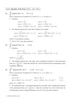
Figure 2 depicts the principal scheme of solving Volterra integral equations of the second kind
with difference kernel by means of the Laplace integral transform.
Page 464
© 1998 by CRC Press LLC
© 1998 by CRC Press LLC
Fig. 2. Scheme of solving Volterra integral equations of the second kind with difference kernel by means
of the Laplace integral transform. R(x) is the inverse transform of the function
˜
R(p)=
˜
K(p)
1 –
˜
K(p)
.
Example 1. Consider the equation
y(x)+A

x
0
sin

λ(x – t)


y(t) dt = f (x), (6)
which is a special case of Eq. (1) for K(x)=–A sin(λx).
We first apply the table of Laplace transforms (see Supplement 4) and obtain the transform of the kernel of the integral
equation in the form
˜
K(p)=–
Aλ
p
2
+ λ
2
.
Next, by formula (4) we find the transform of the resolvent:
˜
R(p)=–
Aλ
p
2
+ λ(A + λ)
.
Furthermore, applying the table of inverse Laplace transforms (see Supplement 5) we obtain the resolvent:
R(x)=





–
Aλ
k

sin(kx) for λ(A + λ)>0,
–
Aλ
k
sinh(kx) for λ(A + λ)<0,
where k = |λ(A + λ)|
1/2
.
Page 465
© 1998 by CRC Press LLC
© 1998 by CRC Press LLC
Moreover, in the special case λ = –A,wehaveR(x)=A
2
x. On substituting the expressions for the resolvent into formula (5),
we find the solution of the integral equation (6). In particular, for λ(A + λ) > 0, this solution has the form
y(x)=f(x) –
Aλ
k

x
0
sin

k(x – t)

f(t) dt, k =

λ(A + λ). (7)
9.3-2. A Method Based on the Solution of an Auxiliary Equation
Consider the integral equation

Ay(x)+B

x
a
K(x – t)y(t) dt = f(x). (8)
Let w = w(x) be a solution of the simpler auxiliary equation with f (x) ≡ 1 and a =0,
Aw(x)+B

x
0
K(x – t)w(t) dt = 1. (9)
In this case, the solution of the original equation (8) with an arbitrary right-hand side can be expressed
via the solution of the auxiliary equation (9) by the formula
y(x)=
d
dx

x
a
w(x – t)f(t) dt = f (a)w(x – a)+

x
a
w(x – t)f

t
(t) dt. (10)
Let us prove this assertion. We rewrite expression (10) (in which we first redenote the integration parameter t by s )in
the form
y(x)=

d
dx
I(x), I(x)=

x
a
w(x – s)f(s) ds (11)
and substitute it into the left-hand side of Eq. (8). After some algebraic manipulations and after changing the order of
integration in the double integral with regard to (9), we obtain
d
dx
AI(x)+B

x
a
K(x – t)
d
dt
I(t) dt =
d
dx
AI(x)+
d
dx
B

x
a
K(x – t)I(t) dt
=

d
dx

A

x
a
w(x – s)f(s) ds + B

x
a

t
a
K(x – t)w(t – s)f(s) ds dt

=
d
dx


x
a
f(s)

Aw(x – s)+B

x
s
K(x – t)w(t – s) dt


ds

=
d
dx


x
a
f(s)

Aw(x – s)+B

x–s
0
K(x – s – λ)w(λ) dλ

ds

=
d
dx

x
a
f(s) ds = f (x),
which proves the desired assertion.
9.3-3. Reduction to Ordinary Differential Equations
Consider the special case in which the transform of the kernel of the integral equation (1) can be

expressed in the form
1 –
˜
K(p)=
Q(p)
R(p)
, (12)
where Q(p) and R(p) are polynomials of degree n:
Q(p)=
n

k=0
A
k
p
k
, R(p)=
n

k=0
B
k
p
k
. (13)
Page 466
© 1998 by CRC Press LLC
© 1998 by CRC Press LLC
In this case, the solution of the integral equation (1) satisfies the following linear nonhomogeneous
ordinary differential equation of order n with constant coefficients:

n

k=0
A
k
y
(k)
x
(x)=
n

k=0
B
k
f
(k)
x
(x). (14)
Equation (14) can be rewritten in the operator form
Q(D)y(x)=R(D)f(x), D ≡
d
dx
.
The initial conditions for Eq. (14) can be found from the relation
n

k=0
A
k
k–1


s=0
p
k–1–s
y
(s)
x
(0) –
n

k=0
B
k
k–1

s=0
p
k–1–s
f
(s)
x
(0) = 0 (15)
by matching the coefficients of like powers of the parameter p.
The proof of this assertion can be performed by applying the Laplace transform to the differential
equation (14) and by the subsequent comparison of the resulting expression with Eq. (2) with regard
to (12).
Another method of reducing an integral equation to an ordinary differential equation is described
in Section 9.7.
9.3-4. Reduction to a Wiener–Hopf Equation of the Second Kind
A Volterra equation of the second kind with the difference kernel of the form

y(x)+

x
0
K(x – t)y(t) dt = f(x), 0 < x < ∞, (16)
can be reduced to the Wiener–Hopf equation
y(x)+

∞
0
K
+
(x – t)y(t) dt = f(x), 0 < x < ∞, (17)
where the kernel K
+
(x – t)isgivenby
K
+
(s)=

K(s) for s >0,
0 for s <0.
Methods for studying Eq. (17) are described in Chapter 11, where an example of constructing
a solution of a Volterra equation of the second kind with difference kernel by means of con-
structing a solution of the corresponding Wiener–Hopf equation of the second kind is presented
(see Subsection 11.9-3).
9.3-5. Method of Fractional Integration for the Generalized Abel Equation
Consider the generalized Abel equation of the second kind
y(x) – λ


x
a
y(t)
(x – t)
µ
dt = f(x), x > a, (18)
Page 467
© 1998 by CRC Press LLC
© 1998 by CRC Press LLC
where 0 < µ < 1. Let us assume that x ∈ [a, b], f (x) ∈ AC, and y(t) ∈ L
1
, and apply the technique
of the fractional integration (see Section 8.5). We set
µ =1– β,0<β <1, λ =
ν
Γ(β)
, (19)
and use (8.5.1) to rewrite Eq. (18) in the form

1 – νI
β
a+

y(x)=f(x), x > a. (20)
Now the solution of the generalized Abel equation of the second kind can be symbolically written
as follows:
y(x)=

1 – νI
β

a+

–1
f(x), x > a. (21)
On expanding the operator expression in the parentheses in a series in powers of the operator by
means of the formula for a geometric progression, we obtain
y(x)=

1+
∞

n=1

νI
β
a+

n

f(x), x > a. (22)
Taking into account the relation (I
β
a+
)
n
= I
βn
a+
, we can rewrite formula (22) in the expanded form
y(x)=f(x)+

∞

n=1
ν
n
Γ(βn)

x
a
(x – t)
βn–1
f(t) dt, x > a. (23)
Let us transpose the integration and summation in the expression (23). Note that
∞

n=1
ν
n
(x – t)
βn–1
Γ(βn)
=
d
dx
∞

n=1
ν
n
(x – t)

βn
Γ(1 + βn)
.
In this case, taking into account the change of variables (19), we see that a solution of the generalized
Abel equation of the second kind becomes
y(x)=f(x)+

x
a
R(x – t)f(t) dt, x > a, (24)
where the resolvent R(x – t) is given by the formula
R(x – t)=
d
dx
∞

n=1

λΓ(1 – µ)(x – t)
(1–µ)

n
Γ[1 + (1 – µ)n]
. (25)
In some cases, the sum of the series in the representation (25) of the resolvent can be found, and a
closed-form expression for this sum can be obtained.
Example 2. Consider the Abel equation of the second kind (we set µ =
1
2
in Eq. (18))

y(x) – λ

x
a
y(t)
√
x – t
dt = f(x), x > a.
(26)
By virtue of formula (25), the resolvent for Eq. (26) is given by the expression
R(x – t)=
d
dx
∞

n=1

λ
√
π(x – t)

n
Γ

1+
1
2
n

. (27)

We have
∞

n=1
x
n/2
Γ

1+
1
2
n

= e
x
erf
√
x, erf x ≡
2
√
π

x
0
e
–t
2
dt, (28)
where erf x is the error function. By (27) and (28), in this case the expression for the resolvent can be rewritten in the form
R(x – t)=

d
dx

exp[λ
2
π(x – t)] erf

λ

π(x – t)


. (29)
Applying relations (24) and (27), we obtain the solution of the Abel integral equation of the second kind in the form
y(x)=f(x)+
d
dx

x
a

exp[λ
2
π(x – t)] erf

λ

π(x – t)



f(t) dt, x > a. (30)
Note that in the case under consideration, the solution is constructed in the closed form.
Page 468
© 1998 by CRC Press LLC
© 1998 by CRC Press LLC
9.3-6. Systems of Volterra Integral Equations
The Laplace transform can be applied to solve systems of Volterra integral equations of the form
y
m
(x) –
n

k=1

x
0
K
mk
(x – t)y
k
(t) dt = f
m
(x), m =1, , n. (31)
Let us apply the Laplace transform to system (31). We obtain the relations
˜y
m
(p) –
n

k=1

˜
K
mk
(p) ˜y
k
(p)=
˜
f
m
(p), m =1, , n. (32)
On solving this system of linear algebraic equations, we find ˜y
m
(p), and the solution of the system
under consideration becomes
y
m
(x)=
1
2πi

c+i∞
c–i∞
˜y
m
(p)e
px
dp. (33)
The Laplace transform can be applied to construct a solution of systems of Volterra equations
of the first kind and of integro-differential equations as well.
•

References for Section 9.3: V. A. Ditkin and A. P. Prudnikov (1965), M. L. Krasnov, A. I. Kiselev, and G. I. Makarenko
(1971), V. I. Smirnov (1974), K. B. Oldham and J. Spanier (1974), P. P. Zabreyko, A. I. Koshelev, et al. (1975), F. D. Gakhov
and Yu. I. Cherskii (1978), Yu. I. Babenko (1986), R. Gorenflo and S. Vessella (1991), S. G. Samko, A. A. Kilbas, and
O. I. Marichev (1993).
9.4. Operator Methods for Solving Linear Integral
Equations
9.4-1. Application of a Solution of a “Truncated” Equation of the First Kind
Consider the linear equation of the second kind
y(x)+L [y]=f(x), (1)
where L is a linear (integral) operator.
Assume that the solution of the auxiliary “truncated” equation of the first kind
L [u]=g(x), (2)
can be represented in the form
u(x)=M

L[g]

, (3)
where M is a known linear operator. Formula (3) means that
L
–1
= ML.
Let us apply the operator L
–1
to Eq. (1). The resulting relation has the form
M

L[y]

+ y(x)=M


L[f]

, (4)
On eliminating y(x) from (1) and (4) we obtain the equation
M [w] – w(x)=F (x), (5)
in which the following notation is used:
w = L [y], F (x)=M

L[f]

– f(x).
In some cases, Eq. (5) is simpler than the original equation (1). For example, this is the case if
the operator M is a constant (see Subsection 11.7-2) or a differential operator:
M = a
n
D
n
+ a
n–1
D
n–1
+ ···+ a
1
D + a
0
, D ≡
d
dx
.

In the latter case, Eq. (5) is an ordinary linear differential equation for the function w.
If a solution w = w(x) of Eq. (5) is obtained, then a solution of Eq. (1) is given by the formula
y(x)=M

L[w]

.
Page 469
© 1998 by CRC Press LLC
© 1998 by CRC Press LLC
Example 1. Consider the Abel equation of the second kind
y(x)+λ

x
a
y(t) dt
√
x – t
= f (x).
(6)
To solve this equation, we apply a slight modification of the above scheme, which corresponds to the case M ≡ const
d
dx
.
Let us rewrite Eq. (6) as follows:

x
a
y(t) dt
√

x – t
=
f(x) – y(x)
λ
.
(7)
Let us assume that the right-hand side of Eq. (7) is known and treat Eq. (7) as an Abel equation of the first kind. Its solution
can be written in the following form (see the example in Subsection 8.4-4):
y(x)=
1
π
d
dx

x
a
f(t) – y(t)
λ
√
x – t
dt
or
y(x)+
1
πλ
d
dx

x
a

y(t) dt
√
x – t
dt =
1
πλ
d
dx

x
a
f(t) dt
√
x – t
.
(8)
Let us differentiate both sides of Eq. (6) with respect to x, multiply Eq. (8) by –πλ
2
, and add the resulting expressions term
by term. We eventually arrive at the following first-order linear ordinary differential equation for the function y = y(x):
y

x
– πλ
2
y = F

x
(x), (9)
where

F (x)=f(x) – λ

x
a
f(t) dt
√
x – t
.
(10)
We must supplement Eq. (9) with initial condition
y(a)=f(a),
(11)
which is a consequence of (6).
The solution of problem (9)–(11) has the form
y(x)=F (x)+πλ
2

x
a
exp[πλ
2
(x – t)]F (t) dt, (12)
and defines the solution of the Abel equation of the second kind (6).
9.4-2. Application of the Auxiliary Equation of the Second Kind
The solution of the Abel equation of the second kind (6) can also be obtained by another method,
presented below.
Consider the linear equation
y(x) – L [y]=f(x), (13)
where L is a linear operator. Assume that the solution of the auxiliary equation
w(x) – L

n
[w]=Φ(x), L
n
[w] ≡ L

L
n–1
[w]

, (14)
which involves the nth power of the operator L, is known and is defined by the formula
w(x)=M [Φ(x)]. (15)
In this case, the solution of the original equation (13) has the form
y(x)=M [Φ(x)], Φ(x)=L
n–1
[f]+L
n–2
[f]+···+ L [f]+f(x). (16)
This assertion can be proved by applying the operator L
n–1
+ L
n–2
+ ···+ L + 1 to Eq. (13), with
regard to the operator relation

1 – L

L
n–1
+ L

n–2
+ ···+ L +1

=1– L
n
together with formula (16) for Φ(x). In Eq. (14) we may write y(x) instead of w(x).
Page 470
© 1998 by CRC Press LLC
© 1998 by CRC Press LLC
Example 2. Let us apply the operator method (for n = 2) to solve the generalized Abel equation with exponent 3/4:
y(x) – b

x
0
y(t) dt
(x – t)
3/4
= f (x). (17)
We first consider the integral operator with difference kernel
L [y(x)] ≡

x
0
K(x – t)y(t) dt.
Let us find L
2
:
L
2
[y] ≡ L


L [y]

=

x
0

t
0
K(x – t)K(t – s)y(s) ds dt
=

x
0
y(s ) ds

x
s
K(x – t)K(t – s) dt =

x
0
K
2
(x – s)y(s) ds,
K
2
(z)=


z
0
K(ξ)K(z – ξ) dξ.
(18)
In the proof of this formula, we have reversed the order of integration and performed the change of variables ξ = t – s.
For the power-law kernel
K(ξ)=bξ
µ
,
we have
K
2
(z)=b
2
Γ
2
(1 + µ)
Γ(2+2µ)
z
1+2µ
. (19)
For Eq. (17) we obtain
µ = –
3
4
, K
2
(z)=A
1
√

z
, A =
b
2
√
π
Γ
2
(
1
4
).
Therefore, the auxiliary equation (14) corresponding to n = 2 has the form
y(x) – A

x
0
y(t) dt
√
x – t
= Φ(x),
(20)
where
Φ(x)=f(x)+b

x
0
f(t) dt
(x – t)
3/4

.
After the substitution A → –λ and Φ → f, relation (20) coincides with Eq. (6), and the solution of Eq. (20) can be obtained
by formula (12).
Remark. It follows from (19) that the solution of the generalized Abel equation with exponent β
y(x)+λ

x
0
y(t) dt
(x – t)
β
= f(x)
can be reduced to the solution of a similar equation with the different exponent β
1
=2β – 1. In
particular, the Abel equation (6), which corresponds to β =
1
2
, is reduced to the solution of an
equation with degenerate kernel for β
1
=0.
9.4-3. A Method for Solving “Quadratic” Operator Equations
Suppose that the solution of the linear (integral, differential, etc.) equation
y(x) – λL [y]=f(x) (21)
is known for an arbitrary right-hand side f (x) and for any λ from the interval (λ
min
, λ
max
). We

denote this solution by
y = Y (f, λ). (22)
Let us construct the solution of the more complicated equation
y(x) – aL [y] – bL
2
[y]=f(x), (23)
Page 471
© 1998 by CRC Press LLC
© 1998 by CRC Press LLC
where a and b are some numbers and f(x) is an arbitrary function. To this end, we represent the
left-hand side of Eq. (23) by the product of operators

1 – aL – bL
2

[y] ≡

1 – λ
1
L

1 – λ
2
L

[y], (24)
where λ
1
and λ
2

are the roots of the quadratic equation
λ
2
– aλ – b = 0. (25)
We assume that λ
min
< λ
1
, λ
2
< λ
max
.
Let us solve the auxiliary equation
w(x) – λ
2
L [w]=f(x), (26)
which is the special case of Eq. (21) for λ = λ
2
. The solution of this equation is given by the formula
w(x)=Y (f, λ
2
). (27)
Taking into account (24) and (26), we can rewrite Eq. (23) in the form

1 – λ
1
L

1 – λ

2
L

[y]=

1 – λ
2
L

[w],
or, in view of the identity (1 – λ
1
L)(1 – λ
2
L) ≡ (1 – λ
2
L)(1 – λ
1
L), in the form

1 – λ
2
L



1 – λ
1
L


[y] – w(x)

=0.
This relation holds if the unknown function y(x) satisfies the equation
y(x) – λ
1
L [y]=w(x). (28)
The solution of this equation is given by the formula
y(x)=Y (w, λ
1
), where w = Y (f , λ
2
). (29)
If the homogeneous equation y(x) – λ
2
L[y] = 0 has only the trivial* solution y ≡ 0, then
formula (29) defines the unique solution of the original equation (23).
Example 3. Consider the integral equation
y(x) –

x
0

A
√
x – t
+ B

y(t) dt = f (x).
It follows from the results of Example 2 that this equation can be written in the form of Eq. (23):

y(x) – AL [y] –
1
π
BL
2
[y]=f(x), L [y] ≡

x
0
y(t) dt
√
x – t
.
Therefore, the solution (in the form of antiderivatives) of the integral equation can be given by the formulas
y(x)=Y (w, λ
1
), w = Y (f, λ
2
),
Y (f , λ)=F(x)+πλ
2

x
0
exp

πλ
2
(x – t)


F (t) dt, F (x)=f(x)+λ

x
0
f(t) dt
√
x – t
,
where λ
1
and λ
2
are the roots of the quadratic equation λ
2
– Aλ –
1
π
B =0.
This method can also be applied to solve (in the form of antiderivatives) more general equations of the form
y(x) –

x
0

A
(x – t)
β
+
B
(x – t)

2β–1

y(t) dt = f (x),
where β is a rational number satisfying the condition 0 < β < 1 (see Example 2 and Eq. 2.1.59 from the first part of the book).
* If the homogeneous equation y(x) – λ
2
L[y] = 0 has nontrivial solutions, then the right-hand side of Eq. (28) must
contain the function w(x)+y
0
(x) instead of w(x), where y
0
is the general solution of the homogeneous equation.
Page 472
© 1998 by CRC Press LLC
© 1998 by CRC Press LLC
9.4-4. Solution of Operator Equations of Polynomial Form
The method described in Subsection 9.4-3 can be generalized to the case of operator equations of
polynomial form. Suppose that the solution of the linear nonhomogeneous equation (21) is given
by formula (22) and that the corresponding homogeneous equation has only the trivial solution.
Let us construct the solution of the more complicated equation with polynomial left-hand side
with respect to the operator L:
y(x) –
n

k=1
A
k
L
k
[y]=f(x), L

k
≡ L

L
k–1

, (30)
where A
k
are some numbers and f(x) is an arbitrary function.
We denote by λ
1
, , λ
n
the roots of the characteristic equation
λ
n
–
n

k=1
A
k
λ
n–k
= 0. (31)
The left-hand side of Eq. (30) can be expressed in the form of a product of operators:
y(x) –
n


k=1
A
k
L
k
[y] ≡
n

k=1

1 – λ
k
L

[y]. (32)
The solution of the auxiliary equation (26), in which we use the substitution w →y
n–1
and λ
2
→λ
n
,
is given by the formula y
n–1
(x)=Y (f, λ
n
). Reasoning similar to that in Subsection 9.4-3 shows
that the solution of Eq. (30) is reduced to the solution of the simpler equation
n–1


k=1

1 – λ
k
L

[y]=y
n–1
(x), (33)
whose degree is less by one than that of the original equation with respect to the operator L. We can
show in a similar way that Eq. (33) can be reduced to the solution of the simpler equation
n–2

k=1

1 – λ
k
L

[y]=y
n–2
(x), y
n–2
(x)=Y (y
n–1
, λ
n–1
).
Successively reducing the order of the equation, we eventually arrive at an equation of the form (28)
whose right-hand side contains the function y

1
(x)=Y (y
2
, λ
2
). The solution of this equation is given
by the formula y(x)=Y (y
1
, λ
1
).
The solution of the original equation (30) is defined recursively by the following formulas:
y
k–1
(x)=Y (y
k
, λ
k
); k = n, , 1, where y
n
(x) ≡ f(x), y
0
(x) ≡ y(x).
Note that here the decreasing sequence k = n, , 1 is used.
9.4-5. A Generalization
Suppose that the left-hand side of a linear (integral) equation
y(x) – Q [y]=f(x) (34)
Page 473
© 1998 by CRC Press LLC
© 1998 by CRC Press LLC

can be represented in the form of a product
y(x) – Q [y] ≡
n

k=1

1 – L
k

[y], (35)
where the L
k
are linear operators. Suppose that the solutions of the auxiliary equations
y(x) – L
k
[y]=f(x), k =1, , n (36)
are known and are given by the formulas
y(x)=Y
k

f(x)

, k =1, , n. (37)
The solution of the auxiliary equation (36) for k = n, in which we apply the substitution y →y
n–1
,
is given by the formula y
n–1
(x)=Y
n


f(x)

. Reasoning similar to that used in Subsection 9.4-3
shows that the solution of Eq. (34) can be reduced to the solution of the simpler equation
n–1

k=1

1 – L
k

[y]=y
n–1
(x).
Successively reducing the order of the equation, we eventually arrive at an equation of the form (36)
for k = 1, whose right-hand side contains the function y
1
(x)=Y
2

y
2
(x)

. The solution of this
equation is given by the formula y(x)=Y
1

y

1
(x)

.
The solution of the original equation (35) can be defined recursively by the following formulas:
y
k–1
(x)=Y
k

y
k
(x)

; k = n, , 1, where y
n
(x) ≡ f(x), y
0
(x) ≡ y(x).
Note that here the decreasing sequence k = n, , 1 is used.
•
Reference for Section 9.4: A. D. Polyanin and A. V. Manzhirov (1998).
9.5. Construction of Solutions of Integral Equations With
Special Right-Hand Side
In this section we describe some approaches to the construction of solutions of integral equations
with special right-hand side. These approaches are based on the application of auxiliary solutions
that depend on a free parameter.
9.5-1. The General Scheme
Consider a linear equation, which we shall write in the following brief form:
L [y]=f

g
(x, λ), (1)
where L is a linear operator (integral, differential, etc.) that acts with respect to the variable x and is
independent of the parameter λ, and f
g
(x, λ) is a given function that depends on the variable x and
the parameter λ.
Suppose that the solution of Eq. (1) is known:
y = y(x, λ). (2)
Let M be a linear operator (integral, differential, etc.) that acts with respect to the parameter λ
and is independent of the variable x. Consider the (usual) case in which M commutes with L.We
apply the operator M to Eq. (1) and find that the equation
L [w]=f
M
(x), f
M
(x)=M

f
g
(x, λ)

, (3)
has the solution
w = M

y(x, λ)

. (4)
By choosing the operator M in a different way, we can obtain solutions for other right-hand

sides of Eq. (1). The original function f
g
(x, λ) is called the generating function for the operator L.
Page 474
© 1998 by CRC Press LLC
© 1998 by CRC Press LLC
9.5-2. A Generating Function of Exponential Form
Consider a linear equation with exponential right-hand side
L [y]=e
λx
. (5)
Suppose that the solution is known and is given by formula (2). In Table 4 we present solutions
of the equation L [y]=f (x) with various right-hand sides; these solutions are expressed via the
solution of Eq. (5).
Remark 1. When applying the formulas indicated in the table, we need not know the left-hand
side of the linear equation (5) (the equation can be integral, differential, etc.) provided that a particular
solution of this equation for exponential right-hand side is known. It is only of importance that the
left-hand side of the equation is independent of the parameter λ.
Remark 2. When applying formulas indicated in the table, the convergence of the integrals
occurring in the resulting solution must be verified.
Example 1. We seek a solution of the equation with exponential right-hand side
y(x)+

∞
x
K(x – t)y(t) dt = e
λx
(6)
in the form y(x, λ)=ke
λx

by the method of indeterminate coefficients. Then we obtain
y(x, λ)=
1
B(λ)
e
λx
, B(λ)=1+

∞
0
K(–z)e
λz
dz. (7)
It follows from row 3 of Table 4 that the solution of the equation
y(x)+

∞
x
K(x – t)y(t) dt = Ax (8)
has the form
y(x)=
A
D
x –
AC
D
2
,
D =1+


∞
0
K(–z) dz, C =

∞
0
zK(–z) dz.
For such a solution to exist, it is necessary that the improper integrals of the functions K(–z) and zK(–z) exist. This
holds if the function K(–z) decreases more rapidly than z
–2
as z →∞. Otherwise a solution can be nonexistent. It is of
interest that for functions K(–z) with power-law growth as z →∞in the case λ < 0, the solution of Eq. (6) exists and is
given by formula (7), whereas Eq. (8) does not have a solution. Therefore, we must be careful when using formulas from
Table 4 and verify the convergence of the integrals occurring in the solution.
It follows from row 15 of Table 4 that the solution of the equation
y(x)+

∞
x
K(x – t)y(t) dt = A sin(λx) (9)
is given by the formula
y(x)=
A
B
2
c
+ B
2
s


B
c
sin(λx) – B
s
cos(λx)

,
B
c
=1+

∞
0
K(–z) cos(λz) dz, B
s
=

∞
0
K(–z) sin(λz) dz.
Page 475
© 1998 by CRC Press LLC
© 1998 by CRC Press LLC
TABLE 4
Solutions of the equation L [y]=f(x) with generating function of the exponential form
No
Right-Hand Side f(x)
Solution y
Solution Method
1

e
λx
y(x, λ)
Original Equation
2
A
1
e
λ
1
x
+ ···+ A
n
e
λ
n
x
A
1
y(x, λ
1
)+···+ A
n
y(x, λ
n
)
Follows from linearity
3
Ax + B
A

∂
∂λ

y(x, λ)

λ=0
+ By(x,0)
Follows from linearity
and the results of row No 4
4
Ax
n
,
n =0,1,2,
A

∂
n
∂λ
n

y(x, λ)


λ=0
Follows from the results
of row No 6 for λ =0
5
A
x + a

, a >0
A

∞
0
e
–aλ
y(x, –λ) dλ
Integration with respect
to the parameter λ
6
Ax
n
e
λx
,
n =0,1,2,
A
∂
n
∂λ
n

y(x, λ)

Differentiation with respect
to the parameter λ
7
a
x

y(x,lna)
Follows from row No 1
8
A cosh(λx)
1
2
A[y(x, λ)+y(x, –λ)

Linearity and relations
to the exponential
9
A sinh(λx)
1
2
A[y(x, λ) – y(x, –λ)

Linearity and relations
to the exponential
10
Ax
m
cosh(λx),
m =1,3,5,
1
2
A
∂
m
∂λ
m

[y(x, λ) – y(x, –λ)

Differentiation with respect
to λ and relation
to the exponential
11
Ax
m
cosh(λx),
m =2,4,6,
1
2
A
∂
m
∂λ
m
[y(x, λ)+y(x, –λ)

Differentiation with respect
to λ and relation
to the exponential
12
Ax
m
sinh(λx),
m =1,3,5,
1
2
A

∂
m
∂λ
m
[y(x, λ)+y(x, –λ)

Differentiation with respect
to λ and relation
to the exponential
13
Ax
m
sinh(λx),
m =2,4,6,
1
2
A
∂
m
∂λ
m
[y(x, λ) – y(x, –λ)

Differentiation with respect
to λ and relation
to the exponential
14
A cos(βx) A Re

y(x, iβ)


Selection of the real
part for λ = iβ
15
A sin(βx) A Im

y(x, iβ)

Selection of the imaginary
part for λ = iβ
16
Ax
n
cos(βx),
n =1,2,3,
A Re

∂
n
∂λ
n

y(x, λ)


λ=iβ
Differentiation with respect
to λ and selection of the real
part for λ = iβ
17

Ax
n
sin(βx),
n =1,2,3,
A Im

∂
n
∂λ
n

y(x, λ)


λ=iβ
Differentiation with respect
to λ and selection of the
imaginary part for λ = iβ
18
Ae
µx
cos(βx)
A Re

y(x, µ + iβ)

Selection of the real
part for λ = µ + iβ
19
Ae

µx
sin(βx)
A Im

y(x, µ + iβ)

Selection of the imaginary
part for λ = µ + iβ
20
Ax
n
e
µx
cos(βx),
n =1,2,3,
A Re

∂
n
∂λ
n

y(x, λ)


λ=µ+iβ
Differentiation with respect
to λ and selection of the real
part for λ = µ + iβ
21

Ax
n
e
µx
sin(βx),
n =1,2,3,
A Im

∂
n
∂λ
n

y(x, λ)


λ=µ+iβ
Differentiation with respect
to λ and selection of the
imaginary part for λ = µ + iβ
Page 476
© 1998 by CRC Press LLC
© 1998 by CRC Press LLC
9.5-3. Power-Law Generating Function
Consider the linear equation with power-law right-hand side
L [y]=x
λ
. (10)
Suppose that the solution is known and is given by formula (2). In Table 5, solutions of the equation
L [y]=f(x) with various right-hand sides are presented which can be expressed via the solution of

Eq. (10).
TABLE 5
Solutions of the equation L [y]=f (x) with generating function of power-law form
No
Right-Hand Side f(x)
Solution y
Solution Method
1
x
λ
y(x, λ)
Original Equation
2
n

k=0
A
k
x
k
n

k=0
A
k
y(x, k)
Follows from linearity
3
A ln x + B
A

∂
∂λ

y(x, λ)

λ=0
+ By(x,0)
Follows from linearity and
from the results of row No 4
4
A ln
n
x,
n =0,1,2,
A

∂
n
∂λ
n

y(x, λ)


λ=0
Follows from the results
of row No 5 for λ =0
5
Ax
n

x
λ
,
n =0,1,2,
A
∂
n
∂λ
n

y(x, λ)

Differentiation
with respect to the parameter λ
6
A cos(β ln x) A Re

y(x, iβ)

Selection of the real
part for λ = iβ
7
A sin(β ln x) A Im

y(x, iβ)

Selection of the imaginary
part for λ = iβ
8
Ax

µ
cos(β ln x)
A Re

y(x, µ + iβ)

Selection of the real
part for λ = µ + iβ
9
Ax
µ
sin(β ln x)
A Im

y(x, µ + iβ)

Selection of the imaginary
part for λ = µ + iβ
Example 2. We seek a solution of the equation with power-law right-hand side
y(x)+

x
0
1
x
K

t
x


y(t) dt = x
λ
in the form y(x, λ)=kx
λ
by the method of indeterminate coefficients. We finally obtain
y(x, λ)=
1
1+B(λ)
x
λ
, B(λ)=

1
0
K(t)t
λ
dt.
It follows from row 3 of Table 5 that the solution of the equation with logarithmic right-hand side
y(x)+

x
0
1
x
K

t
x

y(t) dt = A ln x

has the form
y(x)=
A
1+I
0
ln x –
AI
1
(1 + I
0
)
2
,
I
0
=

1
0
K(t) dt, I
1
=

1
0
K(t)lntdt.
Page 477
© 1998 by CRC Press LLC
© 1998 by CRC Press LLC
9.5-4. Generating Function Containing Sines and Cosines

Consider the linear equation
L [y] = sin(λx). (11)
We assume that the solution of this equation is known and is given by formula (2). In Table 6,
solutions of the equation L [y]=f (x) with various right-hand sides are given, which are expressed
via the solution of Eq. (11).
Consider the linear equation
L [y] = cos(λx). (12)
We assume that the solution of this equation is known and is given by formula (2). In Table 7,
solutions of the equation L [y]=f (x) with various right-hand sides are given, which are expressed
via the solution of Eq. (12).
TABLE 6
Solutions of the equation L [y]=f(x) with sine-shaped generating function
No
Right-Hand Side f(x)
Solution y
Solution Method
1
sin(λx)
y(x, λ)
Original Equation
2
n

k=1
A
k
sin(λ
k
x)
n


k=1
A
k
y(x, λ
k
)
Follows from linearity
3
Ax
m
,
m =1,3,5,
A(–1)
m–1
2

∂
m
∂λ
m
y(x, λ)

λ=0
Follows from the results
of row 5 for λ =0
4
Ax
m
sin(λx),

m =2,4,6,
A(–1)
m
2
∂
m
∂λ
m
y(x, λ)
Differentiation
with respect to the parameter λ
5
Ax
m
cos(λx),
m =1,3,5,
A(–1)
m–1
2
∂
m
∂λ
m
y(x, λ)
Differentiation with respect
to the parameter λ
6
sinh(βx) –iy(x, iβ)
Relation to the hyperbolic
sine, λ = iβ

7
x
m
sinh(βx),
m =2,4,6,
i(–1)
m+2
2

∂
m
∂λ
m
y(x, λ)

λ=iβ
Differentiation with respect
to λ and relation to the
hyperbolic sine, λ = iβ
TABLE 7
Solutions of the equation L [y]=f (x) with cosine-shaped generating function
No
Right-Hand Side f(x)
Solution y
Solution Method
1
cos(λx)
y(x, λ)
Original Equation
2

n

k=1
A
k
cos(λ
k
x)
n

k=1
A
k
y(x, λ
k
)
Follows from linearity
3
Ax
m
,
m =0,2,4,
A(–1)
m
2

∂
m
∂λ
m

y(x, λ)

λ=0
Follows from the results
of row 4 for λ =0
4
Ax
m
cos(λx),
m =2,4,6,
A(–1)
m
2
∂
m
∂λ
m
y(x, λ)
Differentiation
with respect to the parameter λ
5
Ax
m
sin(λx),
m =1,3,5,
A(–1)
m+1
2
∂
m

∂λ
m
y(x, λ)
Differentiation
with respect to the parameter λ
6
cosh(βx) y(x, iβ)
Relation to the hyperbolic
cosine, λ = iβ
7
x
m
cosh(βx),
m =2,4,6,
(–1)
m
2

∂
m
∂λ
m
y(x, λ)

λ=iβ
Differentiation with respect
to λ and relation to the
hyperbolic cosine, λ = iβ
Page 478
© 1998 by CRC Press LLC

© 1998 by CRC Press LLC