The velocities on the right-hand side of this equation are in Fig. 5-2. If the bearing
is stationary and the shaft rotates, the fluid film boundary conditions on the
bearing surface are
U
1
¼ 0; V
1
¼ 0 ð15-2Þ
Under dynamic conditions, the velocity on the journal surface is a vector
summation of the velocity of the journal center, O
1
, and the journal surface
velocity relative to that center. The journal center has radial and tangential
velocity components, as shown in Fig. 15-1. The components are de= dt ¼
Cðde=dtÞ in the radial direction and eðdf=dtÞ in the tangential direction.
Summation of the velocity components of O
1
with that of the journal surface
relative to O
1
results in the following components, U
2
and V
2
(see Fig. 5-2 for the
direction of the components):
U
2
¼ oR þ
de
dt

sin y À e
df
dt
cos y ð15-3Þ
V
2
¼ oR
dh
dx
þ
de
dt
cos y þ e
df
dt
sin y ð15-4Þ
Here, h is the fluid film thickness around a journal bearing, given by the equation
h ¼ C 1 þe cos yðÞ ð15-5Þ
After substitution of U
2
and V
2
as well as U
1
and V
1
in the right-hand side of the
Reynolds equation, Eq. (15-1), the pressure distribution can be derived in a
similar way to that of a steady short bearing. The load components are obtained
by integrating the pressure in the converging clearance only ð0 < y < pÞ as

follows:
W
x
¼À2R
ð
p
0
ð
L=2
0
p cos y dy dz ð15-6Þ
W
y
¼ 2R
ð
p
0
ð
L=2
0
p sin y dy dz ð15-7Þ
Converting into dimensionless terms, the equations for the two load capacity
components (in the X and Y directions as shown in Fig. 15-1) become
W
x
¼À0:5e J
12
jUjþ e
_
ffJ

12
þ
_
ee J
22
ð15-8Þ
W
y
¼þ0:5e J
11
U Àe
_
ffJ
11
À
_
ee J
12
ð15-9Þ
Copyright 2003 by Marcel Dekker, Inc. All Rights Reserved.
Here, the dimensionless load capacity and velocity are
W ¼
C
2
mU
0
L
3
W and U ¼
U

U
0
ð15-10Þ
where U ¼ oR is the time-variable velocity of the journal surface and U
0
is a
reference constant velocity used for normalizing the velocity. The integrals J
ij
and
their solutions are given in Eq. (7-13).
Under steady conditions, the external force, F, is equal to the bearing load
capacity, W . However, under dynamic conditions, the resultant vector of the two
forces accelerates the journal mass according to Newton’s second law:
~
FF À
~
WW ¼ m
~
aa ð15-11Þ
Here, m is the mass of the journal,
~
aa is the acceleration vector of the journal
center,
~
FF is the external load, and
~
WW is the hydrodynamic load capacity. Under
general dynamic conditions,
~
FF and

~
WW are not necessarily in the same direction,
and both can be a function of time. In order to convert Eq. (15-11) to
dimensionless terms, the following dimensionless variables are defined:
m ¼
C
3
U
0
mL
3
R
2
m; F ¼
C
2
mU
0
L
3
F ð15-12Þ
Dividing Eq. (15-11) into two components in the directions of
F
x
and F
y
(along X and Y but in opposite directions) and substituting the acceleration
components in the radial and tangential directions in polar coordinates, the
following two equations are obtained:
F

x
À W
x
¼ m
€
ee À me
_
ff
2
ð15-13Þ
F
y
À W
y
¼Àme
€
ff À 2m
_
ee
_
ff ð15-14Þ
The minus signs in Eq. 15-14 are minus because
F
y
is in the opposite direction to
the acceleration. Here, the dimensionless time is defined as
t ¼ ot, and the
dimensionless time derivatives are
_
ee ¼

1
o
de
dt
;
_
ff ¼
1
o
d
_
ff
dt
ð15-15Þ
Substituting the values of the components of the load capacity, W
x
and W
y
, from
Eqs. (15-8) and (15-9) into Eqs. (15-13) and (15-14), the following two
differential equations for the journal center motion are obtained:
FðtÞcosðf À pÞ¼À0:5e J
12
jUjþJ
12
e
_
ff þ J
22
_

ee þ
m
€
ee À me
_
ff
2
ð15-16Þ
FðtÞsinðf À pÞ¼0:5e J
11
U ÀJ
11
e
_
ff À J
12
_
ee À
me
€
ff À 2m
_
ee
_
ff ð15-17Þ
Copyright 2003 by Marcel Dekker, Inc. All Rights Reserved.
Here, FðtÞ is a time-dependent dimensionless force acting on the bearing. The
force (magnitude and direction) is a function of time. In the two equations, e is
the eccentricity ratio, f is the attitude angle, and
m is dimensionless mass,

defined by Eq. (15-12). The definition of the integrals J
ij
and their solution are in
Chapter 7.
Equations (15-16) and (15-17) are two differential equations required for
the solutions of the two time-dependent functions e and f. The variables e and f
represent the motion of the shaft center, O
1
, with time, in polar coordinates. The
solution of the two equations as a function of time is finally presented as a plot of
the trajectory of the journal center. If there are steady-state oscillations, such as
sinusoidal force, after the initial transient, the trajectory becomes a closed locus
that repeats itself each load cycle. A repeated trajectory is referred to as a journal
center locus.
15.3 JOURNAL CENTER TRAJECTORY
The integration of Eqs. (15-16) and (15-17) is performed by finite differences
with the aid of a computer program. Later, a computer graphics program is used
to plot the journal center motion. The plot of the time variables e and f, in polar
coordinates, represents the trajectory of the journal center motion relative to the
bearing. The eccentricity ratio e is a radial coordinate and f is an angular
coordinate.
Under harmonic conditions, such as sinusoidal load, the trajectory is a
closed loop, referred to as a locus. Under harmonic oscillations of the load, there
is initially a transient trajectory; and after a short time, a steady state is reached
where the locus repeats itself during each cycle.
In heavily loaded bearings, the locus can approach the circle e ¼ 1, where
there is a contact between the journal surface and the sleeve. The results allow
comparison of various bearing designs. The design that results in a locus with a
lower value of maximum eccentricity ratio e is preferable, because it would resist
more effectively any unexpected dynamic disturbances.

15.4 SOLUTION OF JOURNAL MOTION BY
FINITE-DIF FERENCE METHOD
Equations (15-16) and (15-17) are the two differential equations that are solved
for the function of e versus f. The two equations contain first- and second-order
time derivatives and can be solved by a finite-difference procedure. The equations
are not linear because the acceleration terms contain second-power time deriva-
tives. Similar equations are widely used in dynamics and control, and commercial
Copyright 2003 by Marcel Dekker, Inc. All Rights Reserved.
software is available for numerical solution. However, the reader will find it
beneficial to solve the equations by himself or herself, using a computer and any
programming language that he or she prefers. The following is a demonstration of
a solution by a simple finite-difference method.
The principle of the finite-difference solution method is the replacement of
the time derivatives by the following finite-difference equations (for simplifying
the finite difference procedure,
"
FF,
"
mm and
"
tt are renamed F, m and t):
_
ff
n
¼
f
nþ1
À f
nÀ1
2 Dt

;
_
ee
n
¼
e
nþ1
À e
nÀ1
2 Dt
ð15-18Þ
and the second time derivatives are
€
ff
n
¼
f
nþ1
À 2f
n
þ f
nÀ1
Dt
2
;
€
ee
n
¼
e

nþ1
À 2e
n
þ e
nÀ1
Dt
2
ð15-19Þ
For the nonlinear terms (the last term in the two equations), the equation can be
linearized by using the following backward difference equations:
_
ff
n
¼
f
n
À f
nÀ1
Dt
ð15-20Þ
By substituting the foregoing finite-element terms for the time-derivative terms,
the two unknowns e
nþ1
and f
nþ1
can be solved as two unknowns in two regular
linear equations.
After substitution, the differential equations become
F
x

þ
1
2
e
n
J
12
¼ e
n
J
12
f
nþ1
À f
nÀ1
2 Dt

þ J
22
e
nþ1
À e
nÀ1
2 Dt

þ m
e
nþ1
À 2e
n

þ e
nÀ1
Dt
2

À me
n
f
n
À f
nÀ1
Dt

2
ð15-21Þ
F
y
À
1
2
e
n
J
11
¼Àe
n
J
11
f
nþ1

À f
nÀ1
2 Dt

À J
12
e
nþ1
À e
nÀ1
2 Dt

À me
n
f
nþ1
À 2f
n
þ f
nÀ1
Dt
2

À 2m
e
nþ1
À e
nÀ1
2Dt


Â
f
n
À f
nÀ1
Dt

ð15-22Þ
Copyright 2003 by Marcel Dekker, Inc. All Rights Reserved.
Here, F
x
and F
y
are the external load components in the X and Y directions,
respectively. Under dynamic conditions, the load components vary with time:
F
x
¼ FðtÞðcos f À pÞð15-23Þ
F
y
¼ FðtÞðsin f À pÞð15-24Þ
Equations (15-21) and (15-22) can be rearranged as two linear equations in terms
of e
nþ1
and f
nþ1
as follows:
Rearranging Eq. (15-21): A ¼ Be
nþ1
þ Cf

nþ1
ð15-25Þ
Rearranging Eq. (15-22): P ¼ Re
nþ1
þ Qf
nþ1
ð15-26Þ
In the following equations, F and m are dimensionless terms (the bar is omitted
for simplification). The values of the coefficients of the unknown variables [in
Eqs. (15-25) and (15-26)] are
A ¼ F
X
þ
e
n
J
12
2
þ
e
n
J
12
f
nÀ1
2 Dt
þ
J
22
e

nÀ1
2 Dt
þ
2me
n
Dt
2
À
me
nÀ1
Dt
2
þ me
n
f
n
À f
nÀ1
Dt

2
ð15-27Þ
B ¼
J
22
2 Dt
þ
m
Dt
2

ð15-28Þ
C ¼
e
n
J
12
2 Dt
ð15-29Þ
P ¼ F
y
À
e
n
J
11
2
À
e
n
J
11
f
nÀ1
2 Dt
À
J
12
e
nÀ1
2 Dt

À
2me
n
f
n
Dt
2
þ
me
n
f
nÀ1
Dt
2
À
me
nÀ1
f
n
Dt
2
þ
me
nÀ1
f
nÀ1
Dt
2
ð15-30Þ
Q ¼À

e
n
J
11
2 Dt
À
me
n
Dt
2
ð15-31Þ
R ¼À
J
12
2 Dt
À
m
Dt
2
f
n
þ
mf
nÀ1
Dt
2
ð15-32Þ
The numerical solution of the two equations for the two unknowns becomes
e
nþ1

¼
AQ ÀPC
BQ ÀRC
ð15-33Þ
f
nþ1
¼
AR ÀPB
CR ÀQB
ð15-34Þ
Copyright 2003 by Marcel Dekker, Inc. All Rights Reserved.
The last two equations make it possible to march from the initial conditions and
find e
nþ1
and f
nþ1
from any previous values, in dimensionless time intervals of
D
"
tt ¼ oDt.
For a steady-state solution such as periodic load, the first two initial values
of e and f can be selected arbitrarily. The integration of the equations must be
conducted over sufficient cycles until the initial transient solution decays and a
periodic steady-state solution is reached, i.e., when the periodic e and f will
repeat at each cycle.
The following example is a solution for the locus of a short hydrodynamic
bearing loaded by a sinusoidal force that is superimposed on a constant vertical
load. The example compares the locus of a Newtonian and a viscoelastic fluid.
The load is according to the equation
FðtÞ¼800 þ800 sin 2ot ð15-35Þ

In this equation, o is the journal angular speed. This means that the frequency of
the oscillating load is twice that of the journal rotation. The direction of the load
is constant, but its magnitude is a sinusoidal function. The dimensionless load is
according to the definition in Eq. (15-12).
The dimensionless mass is
m ¼100 and the journal velocity is constant.
The resulting steady-state locus is shown in Fig. 15-2 by the full line for a
Newtonian fluid. The dotted line is for a viscoelastic lubricant under identical
FIG. 15-2 Locus of the journal center for the load F
t
¼ 800 þ 800 sin 2ot and journal
mass
m ¼ 100.
Copyright 2003 by Marcel Dekker, Inc. All Rights Reserved.
conditions (see Chapt. 19). The viscoelastic lubricant is according to the Maxwell
model in Chapter 2 [Eq. (2-9)]. The dimensionless viscoelastic parameter G is
G ¼ lo ð15-36Þ
where l is the relaxation time of the fluid and o is the constant angular speed of
the shaft. In this case, the result is dependent on the ratio of the load oscillation
frequency, o
1
, and the shaft angular speed, o
1
=o.
Copyright 2003 by Marcel Dekker, Inc. All Rights Reserved.
16
Friction Characteristics
16.1 INTRODUCTION
The first friction model was the Coulomb model, which states that the friction
coefficient is constant. Recall that the friction coefficient is the ratio

f ¼
F
f
F
ð16-1Þ
where F
f
is the friction force in the direction tangential to the sliding contact
plane and F is the load in the direction normal to the contact plane. Discussion of
the friction coefficient for various material combinations is found in Chapter 11.
For many decades, engineers have realized that the simplified Coulomb
model of constant friction coefficient is an oversimplification. For example, static
friction is usually higher than kinetic friction. This means that for two surfaces
under normal load F, the tangential force F
f
required for the initial breakaway
from the rest is higher than that for later maintaining the sliding motion. The
static friction force increases after a rest period of contact between the surfaces
under load; it is referred to as stiction force (see an example in Sec. 16.3).
Subsequent attempts were made to model the friction as two coefficients of static
and kinetic friction. Since better friction models have not been available, recent
analytical studies still use the model of static and kinetic friction coefficients to
analyze friction-induced vibrations and stick-slip friction effects in dynamic
Copyright 2003 by Marcel Dekker, Inc. All Rights Reserved.
systems. However, recent experimental studies have indicated that this model of
static and kinetic friction coefficients is not accurate. In fact, a better description
of the friction characteristics is that of a continuous function of friction coefficient
versus sliding velocity.
The friction coefficient of a particular material combination is a function of
many factors, including velocity, load, surface finish, and temperature. Never-

theless, useful tables of constant static and kinetic friction coefficients for various
material combinations are currently included in engineering handbooks.
Although it is well known that these values are not completely constant, the
tables are still useful to design engineers. Friction coefficient tables are often used
to get an idea of the approximate average values of friction coefficients under
normal conditions.
Stick-slip friction: This friction motion is combined of short consecutive
periods of stick and slip motions. This phenomenon can take place whenever
there is a low stiffness of the elastic system that supports the stationary or sliding
body, combined with a negative slope of friction coefficient, f, versus sliding
velocity, U, at low speed. For example, in the linear-motion friction apparatus
(Fig. 14-10), the elastic belt of the drive reduces the stiffness of the support of the
moving part.
In the stick period, the motion is due to elastic displacement of the support
(without any relative sliding). This is followed by a short period of relative sliding
(slip). These consecutive periods are continually repeated. At the stick period, the
motion requires less tangential force for a small elastic displacement than for
breakaway of the stiction force. The elastic force increases linearly with the
displacement (like a spring), and there is a transition from stick to slip when the
elastic force exceeds the stiction force, and vice versa. The system always selects
the stick or slip mode of minimum resistance force.
In the past, the explanation was based on static friction greater than the
kinetic friction. It has been realized, however, that the friction is a function of the
velocity, and the current explanation is based on the negative f ÀU slope, see a
simulation by Harnoy (1994).
16.2 FRICTION IN HYDRODYNAMIC AND MIXED
LUBRICATION
Hydrodynamic lubrication theory was discussed in Chapters 4–9. In journal and
sliding bearings, the theory indicates that the lubrication film thickness increases
with the sliding speed. Full hydrodynamic lubrication occurs when the sliding

velocity is above a minimum critical velocity required to generate a full
lubrication film having a thickness greater than the size of the surface asperities.
In full hydrodynamic lubrication, there is no direct contact between the sliding
Copyright 2003 by Marcel Dekker, Inc. All Rights Reserved.
surfaces, only viscous friction, which is much lower than direct contact friction.
In full fluid film lubrication, the viscous friction increases with the sliding speed,
because the shear rates and shear stresses of the fluid increase with that speed.
Below a certain critical sliding velocity, there is mixed lubrication, where
the thickness of the lubrication film is less than the size of the surface asperities.
Under load, there is a direct contact between the surfaces, resulting in elastic as
well as plastic deformation of the asperities. In the mixed lubrication region, the
external load is carried partly by the pressure of the hydrodynamic fluid film and
partly by the mechanical elastic reaction of the deformed asperities. The film
thickness increases with sliding velocity; therefore as the velocity increases, a
larger portion of the load is carried by the fluid film. The result is that the friction
decreases with velocity in the mixed region, because the fluid viscous friction is
lower than the mechanical friction at the contact between the asperities.
The early measurements of friction characteristics have been described by
f –U curves of friction coefficient versus sliding velocity by Stribeck (1902) and
by McKee and McKee (1929). These f –U curves were measured under steady
conditions and are referred to as Stribeck curves. Each point of these curves was
measured under steady-state conditions of speed and load.
The early experimental f –U curves of lubricated sliding bearings show a
nearly constant friction at very low sliding speed (boundary lubrication region).
However, for metal bearing materials, our recent experiments in the Bearing and
Bearing Lubrication Laboratory at the New Jersey Institute of Technology, as well
as experiments by others, indicated a continuous steep downward slope of friction
from zero sliding velocity without any distinct friction characteristic for the
boundary lubrication region. The recent experiments include friction force
measurement by load cell and on-line computer data acquisition. Therefore,

better precision is expected than with the early experiments, where each point was
measured by a balance scale.
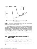
An example of an f –U curve is shown in Fig. 16-1. This curve was
produced in our laboratory for a short journal bearing with continuous lubrica-
tion. The experiment was performed under ‘‘quasi-static’’ conditions; namely, it
was conducted for a sinusoidal sliding velocity at very low frequency, so it is
equivalent to steady conditions. The curve demonstrates high friction at zero
velocity (stiction, or static friction force), a steep negative friction slope at low
velocity (boundary and mixed friction region), and a positive slope at higher
velocity (hydrodynamic region). There are a few empirical equations to describe
this curve at steady conditions. The negative slope of the f –U curve at low
velocity is used in the explanation of several friction phenomena. Under certain
conditions, the negative slope can cause instability, in the form of stick-slip
friction and friction-induced vibrations (Harnoy 1995, 1996).
In the boundary and mixed lubrication regions, the viscosity and boundary
friction additives in the oil significantly affect the friction characteristics. In
Copyright 2003 by Marcel Dekker, Inc. All Rights Reserved.
friction torque is a function of the sliding speed (or viscosity). The current testing
methods for boundary lubricants should be reevaluated, because they rely on the
assumption that there is one boundary-lubrication friction coefficient, indepen-
dent of sliding speed.
For journal bearings in the hydrodynamic friction region, the friction
coefficient f is a function not only of the sliding speed but of the Sommerfeld
number. Analytical curves of ðR=CÞf versus Sommerfeld number are presented
in the charts of Raimondi and Boyd; see Fig. 8-3. These charts are for partial
journal bearings of various arc angles b. These charts are only for the full
hydrodynamic region and do not include the boundary, or mixed, lubrication
region. For a journal bearing of given geometry, the ratio C=R is constant.
Therefore, empirical charts of friction coefficient f versus the dimensionless ratio
mn=P, are widely used to describe the characteristic of a specific bearing. In the

early literature, the notation for viscosity is z, and charts of f versus the variable
zN=P were widely used (Hershey number—see Sec. 8.7.1).
16.2.1 Friction in Roll ing-Element Bearings
Stribeck measured similar f –U curves (friction coefficient versus rolling speed)
for lubricated ball bearings and published these curves for the first time as early as
FIG. 16-2 f –U curve for sinusoidal velocity: oscillation frequency ¼0.05 rad=s,
load ¼37 N, 25-mm journal, L=D ¼0.75, low-viscosity oil, m ¼0.001 N-s=m
2
, no addi-
tives, steel on brass.
Copyright 2003 by Marcel Dekker, Inc. All Rights Reserved.
1902. Rolling-element bearings operating with oil lubrication have a similar
curve: an initial negative slope and a subsequent rise of the friction coefficient
versus speed (due to increasing viscous friction). Although there is a similarity in
the shapes of the curves, the breakaway friction coefficient of rolling bearings is
much lower than that of sliding bearings, such as journal bearings. This is
obvious because rolling friction is lower than sliding friction. The load and the
bearing type affect the friction coefficient. For example, cylindrical and tapered
rolling elements have a significantly higher friction coefficient than ball bearings.
16.2.2 Dry Friction Characteristics
Dry friction characteristics are not the same as for lubricated surfaces. The f –U
curve for dry friction is not similar to that of lubricated friction, even for the same
material combination. For dry surfaces after the breakaway, the friction coefficient
can increase or decrease with sliding speed, depending on the material combina-
tion. For most metals, the friction coefficient has negative slope after the
breakaway. An example is shown in Fig. 16-3 for dry friction of a journal
bearing made of a steel shaft on a brass sleeve. This curve indicates a
considerably higher friction coefficient at the breakaway from zero velocity
(about 0.42 in comparison to 0.26 for a lubricated journal bearing—half of the
breakaway friction). In addition, a dry bearing has a significantly greater gradual

reduction of friction with velocity (steeper slope).
FIG. 16-3 f –U curve for sinusoidal velocity: oscillation frequency ¼0.05 rad=s,
load ¼53 N, dry surfaces, steel on brass, 25-mm journal, L=D ¼0.75.
Copyright 2003 by Marcel Dekker, Inc. All Rights Reserved.
16.2.3 E¡ects of Surface Roughness on Dry
Friction
As already discussed, smooth surfaces are desirable for hydrodynamic and mixed
lubrication. However, for dry friction of metals with very smooth surfaces there is
adhesion on a larger contact area, in comparison to rougher surfaces. In turn,
ultrasmooth surfaces adhere to each other, resulting in a higher dry friction
coefficient. For very smooth surfaces, surface roughness below 0.5 mm, the
friction coefficient f reduces with increasing roughness. At higher roughness,
in the range of about 0.5–10 mm (20–40 microinches), the friction coefficient is
nearly constant. At a higher range of roughness, above 10 mm, the friction
coefficient f increases with the roughness because there is increasing interaction
between the surface asperities (Rabinovitz, 1965).
16.3 FRICTION OF PLASTIC AGAINST METAL
There is a fundamental difference between dry friction of metals (Fig. 16-3)
where the friction goes down with velocity, and dry friction of a metal on soft
plastics (Fig. 16-4a) where the friction coefficient increases with the sliding
velocity. Figure 16-4a is for sinusoidal velocity of a steel shaft on a bearing made
of ultrahigh-molecular-weight polyethylene (UHMWPE). This curve indicates
that there is a considerable viscous friction that involves in the rubbing of soft
plastics. In fact, soft plastics are viscoelastic materials.
In contrast, for lubricated surfaces, the friction reduces with velocity (Fig.
16-4b) due to the formation of a fluid film. In Fig. 16-4b, the dots of higher
friction coefficient are for the first cycle where there is an example of relatively
higher stiction force, after a rest period of contact between the surfaces under
load.
16.4 DYNAMIC FRICTION

Most of the early research in tribology was limited to steady friction. The early
f –U curves were tested under steady conditions of speed and load. For example,
the f –U curves measured by Stribeck (1902) and by McKee and McKee (1929)
do not describe ‘‘dynamic characteristics’’ but ‘‘steady characteristics’’, because
each point was measured under steady-state conditions of speed and load.
There are many applications involving friction under unsteady conditions,
such as in the hip joint during walking. Variable friction under unsteady
conditions is referred to as dynamic friction. Recently, there has been an
increasing interest in dynamic friction measurements.
Dynamic tests, such as oscillating sliding motion, require on-line recording
of friction. Experiments with an oscillating sliding plane by Bell and Burdekin
Copyright 2003 by Marcel Dekker, Inc. All Rights Reserved.
friction model. The amount of hysteresis increases with the frequency of
oscillations. At very low frequency, the curves are practically identical to
curves produced by measurements under steady conditions.
For sinusoidal velocity, the friction is higher during acceleration than
during deceleration, particularly in the mixed friction region. In the recent
literature, the hysteresis effect is often referred to as multivalued friction, because
the friction is higher during acceleration than during deceleration. For example,
the friction coefficient is higher during the start-up of a machine than the friction
during stopping. This means that the friction is not only a function of the
instantaneous sliding velocity, but also a function of velocity history. Examples of
f ÀU curves under dynamic conditions are included in Chap. 17.
Copyright 2003 by Marcel Dekker, Inc. All Rights Reserved.
17
Modeling Dynamic Friction
17.1 INTRODUCTION
Early research was focused on bearings that operate under steady conditions, such
as constant load and velocity. Since the traditional objectives of tribology were
prevention of wear and minimizing friction-energy losses in steady-speed

machinery, it is understandable that only a limited amount of research effort
was directed to time-variable velocity. However, steady friction is only one aspect
in a wider discipline of friction under time-variable conditions. Variable friction
under unsteady conditions is referred to as dynamic friction. There are many
applications involving dynamic friction, such as friction between the piston and
sleeve in engines where the sliding speed and load periodically vary with time.
In the last decade, there was an increasing interest in dynamic friction as
well as its modeling. This interest is motivated by the requirement to simulate
dynamic effects such as friction-induced vibrations and stick-slip friction. In
addition, there is a relatively new application for dynamic friction models—
improving the precision of motion in control systems.
It is commonly recognized that friction limits the precision of motion. For
example, if one tries to drag a heavy table on a rough floor, it would be impossible
to obtain a high-precision displacement of a few micrometers. In fact, the
minimum motion of the table will be a few millimeters. The reason for a low-
precision motion is the negative slope of friction versus velocity. In comparison,
Copyright 2003 by Marcel Dekker, Inc. All Rights Reserved.
one can move an object on well-lubricated, slippery surfaces and obtain much
better precision of motion.
In a similar way, friction limits the precision of motion in open-loop and
closed-loop control systems. This is because the friction has nonlinear character-
istics of negative slope of friction versus velocity and discontinuity at velocity
reversals. Friction causes errors of displacement from the desired target (hang-
off) and instability, such as a stick-slip friction at low velocity.
There is an increasing requirement for ultrahigh-precision motion in
applications such as manufacturing, precise measurement, and even surgery.
Hydrostatic or magnetic bearings can minimize friction; also, vibrations are used
to reduce friction (dither). These methods are expensive and may not be always
feasible in machines or control systems.
An alternate approach that is still in development is model-based friction

compensation. The concept is to include a friction model in the control algorithm.
The control is designed to generate continuous on-line timely torque by the
servomotor, in the opposite direction to the actual friction in the mechanical
system. In this way, it is possible to approximately cancel the adverse effects of
friction. Increasing computer capabilities make this method more and more
attractive. This method requires a dynamic friction model for predicting the
friction under dynamic conditions.
There is already experimental verification that displacement and velocity
errors caused by friction can be substantially reduced by friction compensation.
This effect has been demonstrated in laboratory experiments; see Amin et al.
(1997). Friction compensation has been already applied successfully in actual
machines. For example, Tafazoli (1995) describes a simple friction compensation
method that improves the precision of motion in an industrial machine.
Another application of dynamic friction models is the simulation of
friction-induced vibration (stick-slip friction). The simulation is required for
design purposes to prevent these vibrations.
Stick-slip friction is considered a major limitation for high-precision
manufacturing. In addition to machine tools, stick-slip friction is a major problem
in measurement devices and other precision machines. A lot of research has been
done to eliminate the stick-slip friction, particularly in machine tools. Some
solutions involve hardware modifications that have already been discussed.
These are expensive solutions that are not feasible in all cases. Attempts were
made to reduce the stick-slip friction by using high-viscosity lubricant that
improves the damping, but this would increase the viscous friction losses.
Moreover, high-viscosity oil results in a thicker hydrodynamic film that reduces
the precision of the machine tool. This undesirable effect is referred to as
excessive float.
Copyright 2003 by Marcel Dekker, Inc. All Rights Reserved.
Various methods have been tried by several investigators to improve the
stability of motion in the presence of friction. However, a model-based approach

has the potential to offer a relatively low-cost solution to this important problem.
Armstrong-He
´
louvry (1991) summarized the early work in friction model-
ing of the Stribeck curve by empirical equations. Also, Dahl (1968) introduced a
model to describe the presliding displacement during stiction. However, these
models are ‘‘static,’’ in the sense that the friction is represented by an instanta-
neous function of sliding velocity and load. In recent years, several empirical
equations were suggested to describe the phase lag and hysteresis in dynamic
friction. Hess and Soom (1990) and Dupont and Dunlap (1993) developed such
models.
17.2 DYNAMIC FRICTION MODEL FOR
JOURNAL BEARINGS*
Harnoy and Friedland (1994) suggested a different modeling approach for
lubricated surfaces, based on the physical principles of hydrodynamics. In the
following section, this model is compared to friction measurements. This
approach is based on the following two assumptions:
1. The load capacity, in the boundary and mixed lubrication regions, is
the sum of a contact force (elastic reaction between the surface
asperities) and hydrodynamic load capacity.
2. The friction has two components: a solid component due to adhesion in
the asperity contacts and a viscous shear component.
This modeling approach was extended to line-contact friction by Rachoor and
Harnoy (1996). Polycarpou and Soom (1995, 1996) and Zhai et al. (1997)
extended this approach and derived a more accurate analysis for the complex
elastohydrodynamic lubrication of line contact.
Under steady-state conditions of constant sliding velocity, the friction
coefficient of lubricated surfaces is a function of the velocity. However, under
dynamic conditions, when the relative velocity varies with time, such as
oscillatory motion or motion of constant acceleration, the instantaneous friction

depends not only on the velocity at that instant but is also a function of the
velocity history.
The existence of dynamic effects in friction was recognized by several
investigators. Hess and Soom (1995, 1996) observed a hysteresis effect in
oscillatory friction of lubricated surfaces. They offered a model based on the
steady f –U curve with a correction accounting for the phase lag between friction
and velocity oscillations. The magnitude of the phase lag was determined
empirically. A time lag between oscillating friction and velocity in lubricated
*This and subsequent sections in this chapter are for advanced studies.
Copyright 2003 by Marcel Dekker, Inc. All Rights Reserved.
surfaces was observed and measured earlier. It is interesting to note that
Rabinowicz (1951) observed a friction lag even in dry contacts.
The following analysis offers a theoretical model, based on the physical
phenomena of lubricated surfaces, that can capture the primary effect and
simulate the dynamic friction. The result of the analysis is a dynamic model,
expressed by a set of differential equations, that relates the force of friction to the
time-variable velocity of the sliding surfaces. A model that can predict dynamic
friction is very useful as an enhancement of the technology of precise motion
control in machinery. For control purposes, we want to find the friction at
oscillating low velocities near zero velocity.
Under classical hydrodynamic lubrication theory, (see Chapters 4–7) the
fluid film thickness increases with velocity. The region of a full hydrodynamic
lubrication in the f –U curve (Fig. 16-1) occurs when the sliding velocity is above
the transition velocity, U
tr
required to generate a lubrication film thicker than the
size of the surface asperities. In Fig. 16-1, U
tr
is the velocity corresponding to the
minimum friction. In the full hydrodynamic region, there is only viscous friction

that increases with velocity, because the shear rates and shear stresses are
proportional to the sliding velocity.
Below the transition velocity, U
tr
, the Stribeck curve shows the mixed
lubrication region where the thickness of the lubrication film is less than the
maximum size of the surface asperities. Under load, there is a contact between the
surfaces, resulting in elastic as well as plastic deformation of the asperities. In the
mixed region, the external load is carried partly by the pressure of the hydro-
dynamic fluid film and partly by the mechanical elastic reaction of the deformed
asperities. The film thickness increases with velocity; therefore, as the velocity
increases, a larger part of the external load is carried by the fluid film. The result
is that the friction decreases with velocity in the mixed region, because the fluid
viscous friction is lower than the mechanical friction at the contact between the
asperities.
This discussion shows that the friction force is dependent primarily on the
lubrication film thickness, which in turn is an increasing function of the steady
velocity. However, for time-variable velocity, the relation between film thickness
and velocity is much more complex. The following analysis of unsteady velocity
attempts to capture the physical phenomena when the lubrication film undergoes
changes owing to a variable sliding velocity. As a result of the damping in the
system and the mass of the sliding body, there is a time delay to reach the film
thickness that would otherwise be generated under steady velocity.
17.3 DEVELOPMENT OF THE MODEL
Consider a hydrodynamic journal bearing under steady conditions, when all the
variables, such as external load and speed, are constant with time. Under these
Copyright 2003 by Marcel Dekker, Inc. All Rights Reserved.