540
T.H.T. Chan et al.
density of 7335
kg
/
m 3
and a flexural stiffness EI =
29.97kN/m
2 .
The first three theoretical natural
frequencies of the main beam bridge was calculated as f~ = 4.5
Hz,
f2 = 18.6
Hz,
and f3 = 40.5
Hz.
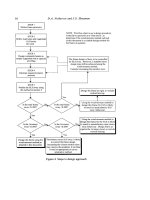
Figure 2. Experimental setup for moving force identification
The U-shape aluminum track was glued to the upper surface of the main beam as a guide for the car.
The model car was pulled along the guide by a string wound around the drive wheel of an electric
motor. The rotational speed of motor could be adjusted. Seven photoelectric sensors were mounted on
the beams to measure and check the uniformity of moving speed of the car. Seven equally spaced
strain gauges and three equally spaced accelerometers were mounted at the lower surface of the main
beam to measure the response. Bending moment calibration was carried out before actual testing
program by adding masses at the middle of the main beam. In addition, a 14-channel type recorder
was employed to record the response signals. Where Channels 1 to 7 were for logging the bending
moment response signals from the strain gauges. Channels 8 to 10 were for the accelerations from the
accelerometers. The channel 11 was connected to the entry trigger. In the meantime, the response
signals from Channels 1 to 7 and Channel 11 were also recorded in the hard disk of personal computer
for easy analysis. The software Global Lab from the Data Translation was used for data acquisition
and analysis in the laboratory test. Before exporting the measured data in ASCII format for
identification calculation, the Bessel IIR digital filters with lowpass characteristics was implemented

as cascaded second order systems. The Nyquist fraction value was chosen to be 0.05.
PARAMETER STUDIES
For practical reason, one parameter was studied at a time. The examination procedure was to examine
one parameter in each case to isolate the case with the highest accuracy for the corresponding
parameter and then another parameter was examined. The parameters, such as the mode number, the
sampling frequency, the speed of vehicle, the computational time, the sensor and sensor locations
were considered as variables to examine their effect on the accuracy of force identification. There are
two ways to check this kind of effects. One is that the identified results are checked
directly
by
comparing the identified forces with the true forces. However, because the true forces are unknown, it
is difficult to proceed. The other way is that the identified results are checked
indirectly
by comparing
the measured responses (bending moments, displacements or accelerations) with the rebuilt responses
calculated from the identified forces. The accuracy is quantitatively defined as Equation (9), called a
Relative Percentage Error (RPE).
RPE = EJftn, e
- ~'dentl
x 100% (9)
El/.el
Equation (9) is also used to calculate the relative percentage errors between the measured and rebuilt
responses from identified forces instead of comparing the identified forces with the true forces
directly. The measured response (R

d) and rebuilt response
(Rreb,,izt)are
herein substituted for the
true force
(ftr,,e)and

identified force
(fide,,)in
equation (9) respectively. In the present parameter
studies, most of results were from the comparison of the relative percentage errors between the
measured and rebuilt response only for the bending moment response. Regarding the results
associated with the accelerations, they will be reported separately.
Parameter Studies of Moving Force Identification in Laboratory
Effects of Mode Number
541
For comparing the effects of different Mode Number (MN) on identified results in the TDM and
FTDM, it was assumed that the sampling frequency (f~) and vehicle speed (c) were constant, and the
case of fs = 250Hz, c = 15
Units
(1.52322
m/s)
was chosen. The data at all the seven measurement
stations for bending moments were employed to identify the moving forces. The mode number was
varied from MN=3 to MN=10. The identified forces were calculated first, and then the rebuilt
responses from the identified forces were then computed accordingly. The Relative Percentage Error
(RPE) for both the TDM and FTDM are shown in Figure 3.
Figure 3. Effects of mode number
For the TDM, the RPE values at the middle measurement stations are always less than the ones at the
two end measurement stations. This is associated with the signal noise ratio of various measurement
stations because there are bigger responses at the middle stations than those at the two end stations. It
is found that when the mode number is equal to or bigger than four, the relative percentage errors are
reduced dramatically. This means the TDM is effective if the required mode number is achieved or
exceeded, otherwise, the TDM will be failed. The minimum RPE value case is of MN=5, the
maximum RPE value case is of the biggest mode number involved (MN=I 0). This also shows that the
case MN=5 is the most optimal case in this kind of comparisons. Similar conclusions are drawn for
the FTDM. However, the biggest difference from the TDM is that the RPE is independent of the

increment MN after MN=5.
By comparing the identification accuracy by the TDM and FTDM in Figure 3, it can be seen that the
results are very close to each other when the MN is equal to 5 and 6 respectively, especially at the
middle measurement stations. However, it can be seen from the identified forces in Figure 4 that the
FTDM is worse than the TDM because it has components with higher frequency noise.
Figure 4. Identified forces (MN=5, fs = 250Hz, c = 15
Units )
Effects of Sampling
Frequency
The sampling frequency fs should be high enough so that there is sufficient accuracy in the discrete
integration in equation (4) and (5) [Law et al 1997]. In the present study, the data was acquired at the
sampling frequency 1000
Hz
per channel for all the cases. This sampling frequency was higher than
the practical demand because only a few of lower frequency modes were usually used in the moving
force identification. Therefore, the sequential data acquired at 1000
Hz
was sampled again in a few
intervals in order to obtain a new sequential data at a lower sampling frequency. Here, a new
542
T.H.T. Chan et al.
sequential data at the sampling frequency of 333,250, and 200
Hz
would be obtained by sampling the
data again every third, fourth and fifth point respectively. For the case of the vehicle running at 15
Units,
the bending moment data was acquired at the different frequencies of 200, 250 and 333
Hz
respectively. The RPE results between the rebuilt and measured bending moment responses are
calculated and listed in Table 1 for both the TDM and FTDM.

TABLE 1
EFFECTS OF SAMPLING FREQUENCY (c = 15
Units)
Sta. TOM FTDM
No. MN=3 MN=4 MN=5 MN=3 MN=4 MN=5
I
II III I II III I II III I II III I II III I II III
1 13.8 783. 412. 6.44 6.05 6.11 8.86 5.32 3.75 188. 1541 1724 6.35 16.1 445. 3.38 4.39 2005
2 7.15 609. 244. 2.81 2.74 2.69 3.34 2.61 2.40 167. 1618 1636 2.68 10.3 419. 2.51 2.16 1370
3 6.50 358. 185. 2.74 2.10 1.95 2.87 2.10 1.94 163. 1679 1647 2.09 8.50 427. 2.01 2.14 1230
4 3.61 216. 216. 3.15 2.96 2.80 3.72 2.71 2.12 165. 1686 1678 2.69 8.05 433. 2.09 2.22 1321
5 6.27 359. 189. 3.16 2.74 2.53 3.58 2.68 2.44 164. 1676 1657 2.61 8.62 430. 2.42 2.13 1238
6 7.41 614. 245. 4.74 4.58 4.32 5.42 4.31 3.45 169. 1615 1654 4.22 10.0 424. 2.89 2.70 1387
7 17.3 780. 420. 6.61 5.84 5.94 9.36 5.19 4.05 187. 1514 1717[ 5.89 16.0 446. 3.92 4.30 2095
Case I, II, and III is for 200,250 and 333 Hz respectively.
For completely comparing the effects of different sampling frequency, the effect of mode number on
identification accuracy is also incorporated in the study. It is found that the higher the sampling
frequency is, the lower the RPE values are for all the measurement stations in the TDM. This shows
that the higher sampling frequency is better than the lower sampling frequency, and the TDM method
has higher identification accuracy if the response is acquired at a higher sampling frequency. In Table
1, it is shown that the FTDM method is failed when the sampling frequency fs = 333
Hz
and mode
number MN=3 because the RPE values are too big to accept for all the measurement stations.
However, The FTDM method is still effective for the case in which the mode number is bigger than 3,
f~ = 200
Hzandf,
= 250
Hz
respectively. By comparing the RPE values at a lower sampling

frequency f~ = 200
Hz
with that at f, = 250
Hz,
it is found that the identification accuracy at
fs = 200
Hz
are higher than one at f, = 250
Hz.
It shows that the identified results are acceptable
and useful if more mode number and suitable sampling frequency is determined in FTDM method.
Effects of Various Vehicle Speeds
In this section, some limitations on identified methods TDM and FTDM should be considered firstly.
In particular, necessary RAM memory and CPU speed of personal computer are required for both the
TDM and FTDM. Otherwise, they will take very long execution time due to the bigger system
coefficient matrix B in equation (7), or they cannot execute at all due to inefficient memory. As the
mode number, the sampling frequency and bridge span length had not been changed for this case, a
change of the vehicle speed would mean a change of the sampling point number, namely change of
dimensions of matrix B in equation (7). Therefore, in order to make TDM and FTDM effective and to
analyze the effects of various vehicle speeds on the identified results, the case of MN=4
and fs = 200
Hz
was selected. When the test was carried out, the three vehicle speeds were set
manually to 5
Units
(0.71224
m/s),
10
Units
(1.08686

m/s),
and 15
Units
(1.52322
m/s)
respectively.
After acquiring the data, the speed of vehicle was calculated and the uniformity of speed was checked.
If the speed was stable, the experiment was repeated five times for each speed case to check whether
or not the properties of the structure and the measurement system had changed. If no significant
change was found, the recorded data was accepted. The RPE values between the rebuilt and measured
bending moment responses are calculated and listed in Table 2. It shows that the TDM is effective for
all the three various vehicle speeds. The RPE values tend to reduce for each measurement station as
the vehicle speed increases. But, the RPE values are close to each other in the case of 10
Units and 15
Parameter Studies of Moving Force Identification in Laboratory
543
Units.
It shows that the identification accuracy for the faster vehicle speed is higher than that at slower
vehicle speed. However, the FTDM is not effective in the case of lower vehicle speed 5
Units,
but the
identified results are getting better and better as the vehicle speed increases. Fortunately, the identified
result is acceptable in the case of 15
Units
in the FTDM.
TABLE 2
EFFECTS OF VEHCILE SPEEDS (MN=4,
fs
= 200Hz )
Station TDM FDTM

No. 5 Units 10 Units 15 Units 5 Units 10 Units 15 Units
1 6.81 5.40 6.45 1045.69 101.53 6.35
2 5.54 2.49 2.81 708.18 46.57 2.68
3 5.88 3.03 2.74 621.36 24.83 2.09
4 8.67 3.01 3.15 562.90 45.11 2.69
5 4.50 2.76 3.16 586.98 23.98 2.61
6 4.66 3.93 4.74 647.38 44.70 4.22
7 6.56 7.94 6.61 965.75 94.26 5.89
Effects of Various Measured Station Number
This section estimates the effects of measurement station number ( N t ) on the identified accuracy. The
N t was set to 2, 3, 4, 5 respectively while the other parameters MN=5, f, = 250
Hz,
c = 15
Units
were not changed. The RPE values between the rebuilt and measured responses are given in Table 3.
The results in Table 3 show that the TDM is required to have at least three measurement stations to
get the two correct moving forces for the front and rear wheel axles respectively. But the FTDM
should have at least one more measurement station, i.e. 4, to get the same moving forces. However,
the errors are increased obviously when the measurement station number is equal to 5 for the FTDM.
TABLE 3
EFFECTS OF MEASUREMENT STATIONS
TDM
Station
No. 2 3 4
1 (L/a) * * *
2 (2L/8) * * 1.50
3 (3L/8) 2003.03 2.15 2.08
4 (4L/8) * 2.27 *
5 (5L/8) 2029.36 2.48 2.04
6 (6L/8) * * 2.38

7 (7L/8) * * *
Asterisk * indicates the station is not chose.
5
1.91
2.21
2.62
2.39
2.82
FTDM
2 3 4 5
* * 2.67
27.06
1192.66 86.92 2.35 14.82
* 115.42 * 27.95
1198.49 87.52 2.49 14.73
* * 2.93 26.62
Comparison of computational time
The computational time consists of three periods, i.e., i) forming the system coefficient matrix B in
equation (7), ii) identifying forces by solving the equation and iii) reproducing the responses. The
above parts are same for the TDM and FTDM. The case described here is of MN=5, f, = 250
Hz,
c = 15 Units,
N t = 7 by using a Pentium II 266 MHz CPU, 64M RAM computer. The total sampling
points are 700 for bending moment response at each measurement station and the total sampling
points are 604 for each wheel axle force in the time domain. Therefore, the dimensions of matrix B are
(7 x 700, 2 • 604). The execution time recorded is listed in Table 4 for the comparison on each period
of the TDM and FTDM in details. It shows that the FTDM takes much longer than the TDM method
in forming the coefficient matrix B. The execution time in other two parts is almost the same for the
two methods. The TDM takes shorter time than the FTDM from the point of view of the total
execution time.

544
T.H.T. Chan et al.
TABLE 4
COMPARISON OF COMPUTATION TIME (in Second)
PERIOD TDM
Forming coefficient matrix B
Identifying forces
Rebuilding responses
Total
FTDM
332.69 1059.57
1837.97 1834.07
55.04 53.99
2225.7 2947.63
CONCLUSIONS
Parameter studies on moving force identification in laboratory test have been carried out in this paper.
These parameters include the mode numbers, the sampling frequencies, the vehicle speeds, the
computational time, the sensor numbers and locations. The study suggests the following conclusions:
(1) A minimal necessary mode number is required for both the TDM and FTDM. It should be equal to
or bigger than 4. If first five modes are determined to identify the moving forces, the identification
accuracy is the highest in the cases studied. (2) The TDM has higher identification accuracy when the
higher sampling frequency is employed. However the FTDM is failed if adopting the higher sampling
frequency and the lower mode number. (3) The faster car speed is of benefit to both the TDM and
FTDM, but FTDM method is not suitable for the slower car speed case. (4) At least three and four
measurement stations are required to identify the two wheel axle forces for the TDM and FTDM
respectively. (5) The TDM takes shorter time than the FTDM. (6) Both the TDM and FTDM can
effectively identify moving forces in time domain and frequency domain respectively, and can be
accepted as a practical application method with higher identification accuracy. (7) From the point of
view of all the parameter effects on the identification accuracy, the TDM is the best identification
method. It should be firstly recommended as a practical method to be incorporated in the future

developed Moving Force Identification System (MFIS).
ACKNOWLEDGMENT
The present project is supported by the Hong Kong Research Grants Council.
REFERENCES
1. Briggs J.C. and Tse M.K. (1992). Impact force Identification using Extracted Modal Parameters and
Pattern Matching. Int. J. Impact Engineering 12:3, 361-372.
2. Chan T.H.T. and O'Connor C. (1990). Wheel Loads from Highway Bridge Strains: Field Studies.
Journal of Structural Engineering 116:7, 1751-1771.
3. Chan T.H.T. Law S.S. Yung T.H. and Yuan X.R. (1999). An Interpretive Method for Moving Force
Identification. Journal of Sound and Vibration 219:3, 503-524.
4. Fryba L. (1972). Vibration of Solids and Structure under Moving Loads, Noordhoff International
Publishing, Prague.
5. Hoshiya M. and Maruyama O. (1987), Identification of Running Load and beam system. Journal of
Engineering Mechanics ASCE, 113, 813-824.
6. Law S.S. Chan T.H.T. and Zeng Q.H. (1997). Moving Force Identification: A Time Domain
Method, Journal of Sound and Vibration, 201:1, 1-22.
7. Law S.S. Chan T.H.T. and Zeng Q.H. Moving Force Identification-Frequency and Time Domain
Analysis, Journal of Dynamic System, Measurement and Control (accepted for publication)
8. Moses F. (1984). Weigh-In-Motion System using Instrumented Bridge, Journal of Transportation
Engineering ASCE, 105(TE3), 233-249.
9. O'Connor C. and Chan T.H.T. (1988). Dynamic Wheel Loads from Bridge Strains, Journal of
Structural Engineering, 114:8, 1703-1723.
10.Stevens K. K. (1987). Force Identification Problems-An Overview, Proceeding of SEM Spring
Conference on Experimental Mechanics, 838-844.
SEISMIC ANALYSIS OF ISOLATED
STEEL HIGHWAY BRIDGE
Xiao-Song LI 1 and Yoshiaki GOTO 2
1 Research Associate, 2 Professor
Dept. of Civil Engineering, Nagoya Institute of Technology
Gokiso-cho, Showa-ku, Nagoya 466-8555, Japan

ABSTRACT
Seismic isolators with dissipation devices have been widely used for highway bridges in Japan,
because they may effectively absorb energy and reduce inertia force induced by earthquake. The main
factors that influence the response of the isolated bridge are initial stiffness and yield force of the
isolator. These quantities should be appropriately designed. Besides, introduction of the isolators leads
to an interaction between the bridge pier and the isolator and increases the computational difficulty
due to the nonlinearity that occurs in both the pier and the isolator. The purpose of this paper is to
investigate the seismic response of the isolated bridges subjected to ground motions, where we
examine how the behaviors of the bridge pier are influenced by the initial stiffness and yield force of
the isolator and the elongation of natural period of the bridge. Then, the applicability of the
'Displacement Conservation Principle' for predicting the maximum responses of the piers of the
isolated steel bridges is numerically examined. The numerical results show that the application of the
'Displacement Conservation Principle' may be reasonably safe and accurate for the practical design of
isolated steel piers.
KEYWORDS
seismic isolation design, nonlinear dynamic analysis, steel highway bridge
545
546
INTRODUCTION
X S. Li and Y. Goto
After the great earthquake happened in Kobe, in 1995, seismic isolators with dissipation devices have
been widely used for highway bridges in Japan. Due to the significant increase of the natural period,
the isolators may effectively absorb energy and reduce inertia force induced by earthquake. The main
factors that influence the response of the isolated bridge are initial stiffness and yield force of the
isolator. These quantities should be appropriately designed. Besides, introduction of the isolators leads
to an interaction between the bridge pier and the isolator and increases the computational difficulty
due to the nonlinearity that occurs in both the pier and the isolator. The purpose of this paper is to
investigate the seismic response of the isolated bridges subjected to ground motions, where we
examine how the behaviors of the bridge pier are influenced by the initial stiffness and yield force of
the isolator and the elongation of natural period of the bridge. Then, the applicability of the

'Displacement Conservation Principle' for predicting the maximum responses of the piers of the
isolated steel bridges is numerically examined. The numerical results show that the application of the
'Displacement Conservation Principle' may be reasonably safe and accurate for the practical design of
isolated steel piers.
ANALYTICAL MODEL
A typical isolated bridge is used as an analytical model, as shown in Fig.1. The total weight of the
bridge M=1067ton consists of the weight of the deck Mb=0.95M and the weight of the pier Mp=0.05M.
For the height of piers, two values are considered, that is, H=13m for Model-l, and H=11m for
Model-2. The corresponding fundamental natural periods for the two piers are Tl=0.705s and
T2=0.549s.
Fig.l: Analytical Model
A lead-rubber bearing (LRB) is assumed as an isolator with dissipation device that has bilinear yield
stiffness as shown in Fig.2. In Fig.2, Qy and Uby are the yield force and yield displacement,
Seismic Analysis of Isolated Steel Highway Bridge
547
respectively. K~,~ and
Kb2 are
the elastic stiffness and post-yield stiffness with a relation of
Kbz=KbJ6.5;
Kr~ is the equivalent stiffness and
UBe=0.7Ub
which are suggested by the 'Manual of Menshin
(isolation and dissipation) Design of Highway Bridges' (1992).
Fig.2: Hysteresis Behavior of Isolator
ANALYTICAL METHOD
A numerical method that considers both geometrical and material nonlinearity is used to carry out the
dynamic analysis (Li and Goto, 1998). The post-yield modulus of material is assumed to be Ep=E/100.
The effect of damping is considered by a mass-proportional damping matrix. The damping coefficient
is set to h=0.01 for elasto-plastic analysis and h 0.05 for elastic analysis.
Two standard ground accelerations suggested by Japan Road Association are used for the analysis.

One is Type 2 at Soil Group II (hard soil site), the other is Type 2 at Soil Group Ill (soft soil site).
Both acceleration waves are illustrated in Fig.3. The time interval adopted in the numerical integration
is 0.01s.
Fig.3: Ground Accelerations
In order to investigate the effect of the initial stiffness and yield force of the isolator, the calculation is
carried out by changing
Qy/Py
and I~I/K p from 0.2 to 0.9 that is the possible range in practical design,
where Py=2( cr y-Mg/A)/(HB) and Kp=3EI/H 3 are the yield force and elastic stiffness of the pier.
548
NUMERICAL RESULTS
X S. Li and Y. Goto
Typical responses of an isolated bridge are shown in Fig.4. It can be seen from Fig.4 (a) that the
displacement of the pier is much smaller than that of the deck due to the isolator. Furthermore, the pier
is damaged little and the energy induced by seismic wave is almost dissipated in the isolator, as
illustrated in Fig.4 (b). In the following, the effects of the initial stiffness Kb~ and yield force
Qy of the
isolator and the elongation of natural period of the bridge are investigated. Then, the applicability of
the 'Displacement Conservation Principle' for predicting the maximum responses of the piers of the
isolated steel bridges is numerically examined.
Fig.4: Responses of Model-1 with Qy/Py=0.6 and Kbl/I~ =0.5 Subjected to Wave Type 2-111
Effect of K~l and Qy on Pier and Isolator
With the designated yield force ratios Qy/Py=0.3, 0.5 and 0.7, the maximum response displacements of
the pier and the isolator are obtained by changing the initial stiffness ratio Kbl/Kp from 0.2 to 0.9. The
relations of ductility factors//p and/1 b of the pier and the isolator vs. the initial stiffness ratio Kb~/K p
of the isolator are shown in Fig.5 for Model-1 and Model-2 subjected to waves Type 2-II and Type
2-lit. In this figure, the ductility factors for piers and isolators are defined as /1
p=Upmax/Upy
(with solid
line) and /1

b=Ubmax/Uby
(with dotted line), where Upmax=maximum displacement of pier, Upy=yield
displacement of pier, and Ubmax=maximum displacement of isolator and Uby=yield displacement of
isolator. It should be noted that the/1
p
may be considered as the maximum response or the ductility
factor of the pier, while/.t b denotes only the ductility factor of the isolator because the
Uby
varies with
Qy/Py or Kb~/K p. Similarly, the relations that vary with the yield force ratio Qy/Py are shown in Fig.6 for
the designated initial stiffness ratios Kbl/Kp=0.3, 0.5 and 0.7.
From Fig.5, it can be seen that the both ductility factors ~t p and /~ b of the pier and the isolator
increase with the increase of the initial stiffness ratio
Kbl/K. p
of the isolator for all cases. However,
Seismic Analysis of Isolated Steel Highway Bridge
549
some influences caused by the wave types can be found as follows. The maximum responses of the
pier subjected to wave Type 2-11" almost linearly increase
as Kbl/Kp
increases from 0.2 to 0.9 as
shown in Fig.5(a), while those subjected to wave Type 2-m" increase a little shapely when Kbl/I~ >0.6.
Furthermore, the values of It p for Model-2 with a smaller ratio of Qy/Py=0.3 become greater than
those with Qy/Py=0.5 and 0.7 when Kbl/Kp~0.6, as shown in Fig.5(c). The relations between the
ductility factor It b of the isolator and Kbl/Kp exhibit a different tendency depending on the value of
Qy/Py. That is, It b with Qy/Py=0.3 exhibits a large increase, while that with Qy/Py=0.7 shows just a
small increase.
Fig.5: Effect of Initial Stiffness Ratio Kbl/Kp of Isolator on Ductility Factors It
p
and It b

Fig.6: Effect of Yield Force Ratio Qy/Py of Isolator on Ductility Factors It
p
and It b