310 M. Saidani et al.
were observed: (a) weld fracture; (b) tube yield failure; (c) local fracture of the tube wall at the
vicinity of the weld.
Failure mode (a) would only occur if the weld were the weakest part of the joint. This could be
avoided by carefully controlling the quality (and size) of the weld. Failure mode (b) is the more
general one, occurring in almost all the tests. If the welds in the cap plate-tube connection and the
cleat plate-tube connection are strong, then failure mode (c) may take place especially for
connections with thinner plates. As can be seen from Figure 5, the axial deformation remains linear
for load of up to 230kN (estimated first yield point). In this case, the failure load was 313kN. This
gives a ratio of ultimate strength to yield strength of 1.36. In reality the ultimate load could be
higher since the test was stopped as soon as the machine ceased taking any more loads. The stresses
at mid-height of the tube (Figure 6) were linear up to about 120kN and thereafter non-linear. This
was typical in all the specimens tested. Good agreement is obtained with the finite element
modelling as shown in the companion paper, Karadelis et al (1999).
Load (kN)
35O
30O
250
2OO
150
100
50
0
0
10 20 30
Overall axial deformation(mm)
Figure 5: Load vs axial deformation (LVDT1)
Load (kN)
35O
3O0
25O

20O
150
100
5O
0
I
i i
0 200 400 600 800
Stress in tube (N/mm 2)
Figure 6: Load vs axial stress in the tube (SG2/3)
35o ] Load (kN)
300 J~
250 ff
200 ~1
150
100
-50 0
50
Out-of-plane bending moment (kN.m)
-10 -5
350
300
250
200
150
100
50
0
0 5
In-plane bending moment (kN.m)

Figure 7" Load vs out-of-plane bending
Figure 8: Load vs in-plane bending
It is also evident from Figures 6 (and in fact in other specimens), that extensive stress redistribution
and strain hardening were taking place. Examination of Figures 7 and 8 show that the in-plane and
Behaviour of T-End Plate Connections to RHS Part I 311
out-of-plane bending moments were small and could therefore be ignored. As the load approaches
the failure load, the deformations in the specimen become more important resulting in a sharp
increase in in-plane and out-of-plane bending moments. Again, this was characteristic in all the
joints tested.
CONCLUSIONS AND FUTURE WORK
The behaviour of welded T-end plate connections has been investigated through a series of tests.
Numerical models have also been used to predict their behaviour. It was found that, apart from any
weld defects, the mode of failure of the joint could be by generalised tube yielding or local fracture
of the tube wall. It is suspected that as the cap plate gets thicker (more than 25mm), the capacity of
the joint is reduced suggesting that joints with excessively thicker plates are less stronger than
would normally be expected. The results also suggest that considerable stress re-distribution and
strain hardening were taking place after the first yield More tests are under way for 'true' rectangular
hollow section tubes (as compared to square). The effect of changing the orientation of the cap plate
in relation to the tube will be examined. The finite element model will be further refined and
benchmarked. The results will be used to produce design guideline for this type of connection,
based on this work but also on previous published work.
AKNOWLEDGEMENTS
The authors are very grateful for the generous support and contribution from British Steel, pipes and
tubes (Corby, UK), especially to Mr Eddie Hole, sales manager, and Noel Yeomans, technical
manager. Thanks also to Mr John Griffiths for his assistance is preparing and testing the specimens.
REFERENCES
Cran J.A. (1977). World wide applications of structural hollow sections, the sky's the limit.
Symposium on tubular structures, Delft, The Netherlands, 23.1-23.14.
Comite International pour le Developpement et l'Etude de la Construction Tubulaire, British Steel,
and the Commission of the European Communities (1984). Construction with hollow sections,

Wellingborough, Northants, UK.
Packer J.A., Wardenier J., Kurobane Y., Dutta D., and Yeomans N. (1992). Design guide for
rectangular hollow section (RHS) joints under predominantly static loading. Verlag TUV,
Rheinland, Koln, Germany.
Kitipornchai S. and Traves W.H. (1989). Welded T-end connections for circular hollow tubes.
Structural Engineering, ASCE 115:12, 3155-3170.
Stevens N.J. and Kitipornchai S. (1990). Limit analysis of welded tee end connections for hollow
tubes. Structural Engineering, ASCE 116:9, 2309-2323.
Granstrom A. (1979). End plate connections for rectangular hollow sections. The Swedish Steel
Construction Institute. Report 15:15.
Karadelis J.N., Saidani M., Omair M.R. (1999). Behaviour of end-plate connection to rectangular
hollow section. Part II: Numerical modelling. ICASS99', Hong Kong, PRC.
This Page Intentionally Left BlankThis Page Intentionally Left BlankThis Page Intentionally Left BlankThis Page Intentionally Left BlankThis Page Intentionally Left BlankThis Page Intentionally Left BlankThis Page Intentionally Left BlankThis Page Intentionally Left BlankThis Page Intentionally Left BlankThis Page Intentionally Left BlankThis Page Intentionally Left BlankThis Page Intentionally Left BlankThis Page Intentionally Left BlankThis Page Intentionally Left Blank
THE BEHAVIOUR OF T-END PLATE CONNECTION TO SHS.
PART II: A NUMERICAL MODEL
J N Karadelis, M Saidani, M Omair.
School of the Built Environment, Coventry University,
Coventry, CV 1 5FB, UK.
ABSTRACT
The behaviour and performance of a family of structural connections made of square hollow sections
(SHS) has been investigated in the laboratory and a series of data have been collected and presented
in a graphical form. In parallel, a rigorous finite element model was developed capable of analysing
the system of the SHS, the cap-plate, the cleat-plate and its surrounding weld. Evidence of non-
linearity and deviation from the classical linear elastic theory led to a more complex numerical
solution to fit more closely the experimental data. A specific methodology is presented, as it applies
to analyses involving plasticity and large deflections (deformations). Test results obtained in the
laboratory were compared with computed values from the finite element analysis and are presented
graphically in the last pages of this paper. Satisfactory agreement was obtained between recorded and
computed strains and displacements. The paper includes extensive discussion of the above results
and the conclusions drawn from them. A brief account of directly related future research work is also

given.
KEYWORDS
SHS, Non-linear, FE-Analysis, ANSYS, Stresses, Strains, Displacements.
INTRODUCTION
There is no doubt that the description of non-linear phenomena inevitably lead to non-linear
equations which immediately render classical methods of mathematical analysis inapplicable. No
method is yet known for finding the exact solution to a system of non-linear equations, such as the
one shown below.
{Fe}=[ke(8,F)]{8 ~}
(1)
Where:
[ke(8,F)] = stiffness matrix of the element which is a function of {8} and {F}.
{8 e} = displacement vector of the element.
{F e} = load vector of the element.
313
314
J.N. Karadelis et al.
Non linear structural behaviour arises from a number of phenomena, which can be grouped into three
main categories such as, changing status, geometric non-linearities and material non-linearities.
THEORY
Due to their nature, non-linear problems require special solution techniques. The established
Newton-Raphson (N-R) method, Zienkiewicz O C et at (1994) is a series of successive linear
approximations (iterations) with corrections and can be used in special algorithms to solve non-linear
problems. The stiffness matrix [K] and the restoring force {F nr} vary with the applied load. Each
linear approximation requires at least one iteration through the equation solver. The stiffness matrix
[K] may be updated in every iteration, occasionally, or not at all. Accordingly, the method is called
full, modified, or initial-stiffness (N-R) procedure.
GEOMETRIC NON-LINEARITIES (LARGE DISPLACEMENTS APPROACH).
If a structure undergoes large displacements as the load is applied incrementally, then the stiffness
matrix will not be constant during the loading process. When a small tensile load is applied at the

centre of the cap-plate welded around the periphery of a square hollow steel member (Figure 1, end
of paper), the strain energy stored in the material is due to bending of the plate only. However, when
the load becomes large enough to bow the plate significantly, the area of the plate around the line of
application of the load will undergo further deformation to accommodate the additional strain.
Therefore, the stiffness of the plate at this central region will increase. From the finite element point
of view, geometric non-linearities are not difficult to deal with, provided that stresses do not affect
the stiffness matrices significantly (that is, the stiffness matrices formed are not stress dependant).
In a typical case like the above, the load was divided into a series of sufficiently small increments
(steps) and these were applied one at a time. ANSYS strongly recommends that for large
displacements analyses the loads specified in the load steps should be 'stepped up' (as opposed to
'ramped on'). This means that the value of a particular load step will be reached during the first
iteration and will be kept constant during the remaining iterations, until the end of the load step. This
contributes to faster convergence. After each increment the deflections caused were calculated by
using the linear version of the equation 1, above. That is, it was assumed that the stiffness matrix was
constant during the application of each load increment. The initial stiffness matrix was used to
generate the equations for the next increment and so on, until the process was completed. The
original co-ordinates of the nodes were then shifted by an amount equal to the values of the
displacements calculated. The new stiffness matrix for the deformed plate was re-calculated and the
process was repeated until the total load was reached. The matrix notation of the incremental
procedure, using the linear version of the equation 1 above, is shown below.
{AF, }= [K
(i-1)]{ A
ai},
V i ~ 9t N :i = 1,2,3,4,
(2)
(i= positive integer representing stage of incremental loading)
The initial Tangent Modulus, tE0, was taken from a non-linear stress-strain curve obtained from
experimental observations. The initial stiffness matrix [K0], was then computed from the tangent
modulus tE0 and the Poisson's Ratio, v. Note that v could also be defined as Tangent Poisson's ratio
tv0 and can be obtained by evaluating the first derivative of the volumetric strain with respect to the

axial strain curve. However, this was not found to be appropriate at this stage.
The Behaviour of T-End Plate Connections to SHS. Part
H 315
It is important to keep the load increments small, so that the increments in displacement cause
negligible changes in the stiffness matrix at each step. On the other hand, increments should be
sufficiently large otherwise the cost of computer running may become excessive. These
displacements were added together and gave the total displacement after the final increment. Stresses
and strains corresponding to the above displacements were treated in the same manner.
ANSYS activates the large deflection analysis within the static analysis using the
NLGEOM, ON
option. It can be summarised as a three step process for each element.
1. Determination of the updated transformation matrix [Tn] for the element.
2. Extraction of the deformation displacement {Und}, from the total element displacement {Un}, in
order to compute the stresses and the restoring force {Fenr}.
3. After the rotational increments in {Au} are computed, node rotations must be updated
Any desired loading can be applied. However, the program must be allowed to iterate until the
solution converges. Intermediate iterations are not in equilibrium and do not represent valid
solutions. In order to obtain valid solutions at intermediate load levels, and/or to observe the structure
under different loading configurations, multiple load steps may be desired.
A synoptical flow chart containing the main steps for large displacements analysis and demonstrating
the presence of stress stiffening effects is shown below, in Figure 2. Simply stated, stress stiffening
looks at the state of stress in a FE-model and calculates a stiffness matrix, [S], based upon it. Matrix
[S] is then added to the usual (initial) matrix [K] and a new set of displacements are calculated.
Form
K
Calculate
u0
and stresses.
Calculate S
from stress

state and
add to K
V3
First iteration
Second and subsequent
iterations.
316
J.N. Karadelis et al.
Calculate
displacements
and stresses using
(K+Si)
Ui-
F
Yes
J
STOP
Second and subsequent
iterations.
)
Figure:
2 The basic steps of a non-linear, large displacements analysis
MATERIAL NON-LINEARITIES
Material non-linearities occur when the stress is a non-linear function of the strain. The relationship
is also path dependant, that is, the stress depends on the strain history as well as the strain itself.
ANSYS accounts for several types of material non-linearities. Rate independent plasticity will be
utilised here as it is characterised by irreversible straining, once a certain level of stress is reached.
Elasto-plastic behaviour. General approach.
ANSYS theory for elasto-plastic analysis, provides the user with three main elements: The yield
criterion, the flow rule and the hardening rule.

The yield criterion determines the stress level at which yielding is initiated. For two and three
dimensional stress systems this can be interpreted through the equivalent stress (~eq), MASE G E
(1970). The flow rule determines the direction of plastic straining (ie: which direction the plastic
strains flow) relative to x,y,z axes. Finally, the hardening rule describes the changes the yield surface
undergoes with progressive yielding so that the various states of stress for subsequent yielding can be
established. For an assumed perfectly plastic material the yield surface does not change during
plastic deformation and therefore the initial yield condition remains the same. For a strain hardening
material, however, plastic deformation is generally accompanied by changes in the yield surface.
Two hardening rules are available and these are isotropic (work) hardening and kinematic hardening.
The Behaviour of T-End Plate Connections to SHS. Part H
Multilinear Isotropic Hardening
317
For materials with isotropic plastic behaviour, the assumption of isotropic hardening under loading
conditions postulates that, as plastic strains develop, the yield surface simply increases in size and
maintains its original shape. ANSYS, uses the von Mises yield criterion with the associated flow rule
and isotropic (work) hardening. When the equivalent stress is equal to the current yield stress the
material is assumed to undergo yielding. The yield criterion is known as the 'work hardening
hypothesis' and assumes that the current yield surface depends only upon the amount of plastic work
done.
The solutions of non-linear elastic and elasto-plastic materials are usually obtained by using the
linear solution, modified with an incremental and iterative approach. The material is assumed to
behave elastically before reaching yield as defined by Hooke's low. If the material is loaded beyond
yielding, then additional plastic strains will occur. They will accumulate during the iteration process
and after the removal of the load will leave a residual deformation.
In general:
~ ~n(ela) "q- iCn(pla) nt" ~
(3)
where:
en = total strain for the current iteration.
lgn(ela) =

elastic strain for the current iteration.
Agn(pla) =
additional plastic strain obtained from the same iteration.
gn-l(pla) =
total, previously obtained plastic strain.
Convergence is achieved when
Agn(pla)/gn(ela)
is less than a criterion value, Walz J E et al (1978). This
means that very little additional plastic strain is accumulating and therefore the theoretical curve is
very close to the actual one.
For the case of uniaxial tension, it is necessary to define the yield stress and the stress-strain
gradients after yielding. For the uni-axial stress governing the SHS member alone, these are simply
Crxx and exx. When Oxx becomes greater than the uniaxial yield stress then yielding takes place. The
yield condition
G'xx > (5"yield
(4)
is the well established von Mises yield criterion for one dimensional state of stress.
Typically, a set of flow equations (flow rule) can be derived from the yield criterion which imply that
the plastic strains develop in a direction normal to the surface (associative rule). The associative flow
rule for the von Mises yield criterion is a set of equations called the incremental Prandtl-Reuss flow
equations MASE G E (1970). That is, the strain increment is split into elastic and plastic portions and
the plastic strain increments are dependant on the deviator stresses. Hence, it is necessary to apply
the total load on the structure in increments. These load steps need only start after the FE-model is
loaded beyond the point of yielding. The size of the subsequent load steps depends on the problem.
The load increments will continue until the total load has been reached or until plastic collapse of the
structure has occurred.
318 J.N. Karadelis et al.
As the load increases the plastic region spreads in the structure and the non-linear problem is
approached using the full Newton-Raphson procedure. The stiffness used in the N-R iterations is the
tangent stiffness and reflects the softening of the material due to plasticity. It should be noted that in

general, the flatter the plastic region of the stress-strain curve, the more the iterations needed for
convergence.
As plasticity is path dependant or a non-conservative phenomenon, it requires that in addition to
multiple iterations per load step the loads be applied slowly, in increments, in order to characterise
and model the actual load history. Therefore, the load history needs to be discretised into a number of
load steps with the presence of convergence tests in each step. ANSYS recommends a practical rule
for load increment sizes such as the corresponding additional plastic strain does not exceed the order
of magnitude of the elastic strain. That is, the plasticity ratio:
Ae"(Pta) ___ 5 (5)
Cn(ela)
In order to achieve inequality 9, the following loading sequence was adopted:
Load step one was chosen so that to produce maximum stresses approximately equal to yield stress
The yield stress was estimated from the experimental stress-strain curves and validated by
performing a linear run with a unit load and by restricting the stresses to the critical stress of the
material. This was found to be approximately equal to 200 kN. Successive load steps were chosen
such as to produce additional plastic strain of the same magnitude as the elastic strain or less. This
was achieved by applying additional load increments no larger that the load in step one, scaled by the
ratio ET]E. Such as:
E T
P~+, = E P~ Vn~9~ N
(6)
where:
E = Elastic slope
Ev = Plastic slope
with: Ev/E not less than 0.05
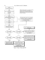
Table 1 below summarises the plasticity theory that characterises the elasto-plastic response of a
certain type of materials. However, the basic steps characterising a non-linear elasto-plastic analysis
are shown in a brief flow chart, in Figure 3.
Material Option
Multi-linear

Isotropic
Hardening
Yield Criterion
von Mises
Flow Rule
Associative
(Prandtl-Reuss
equations)
Hardening
Rule
Isotropic
Material
Response
Multilinear
Table: 1 Summary of the theories involved in a material with multi-linear isotropic
hardening behaviour.
(
The Behaviour of T-End Plate Connections to SHS. Part H
(START)
Form
K
Calculate
u0~
(5"0, ~0
No.
(Linear elastic)
STOP -')
Load Step 1
\.75/
~

Yes. (proceed with nonlinear analysis)
I Calculate "~
AUl, AG1 and AE:I
" and add to
u0~
(Y0~ ~;0
Calculate
displacements
and stresses and add to
previous values.
Yield Criterion
Is ~
~~
Load=Tgt.Load
9 jJ
~
Yes
( )
319
Incremental Procedure
and repeated Iterations.
Figure: 3 The basic steps of a non-linear, elasto-plastic analysis