356 Sinusoidal Steady-State Analysis
9.67 The op amp in the circuit seen in Fig. P9.67 is ideal.
PSPICE Find the steady-state expression for v
(>
(t) when
- =2cosl(/Y V
Figure P9.67
too
kn
40 kO
9.68 The op amp in the circuit in Fig. P9.68 is ideal.
MULTISIM
a
) ^
n<
^ ^
e stea
dy-state expression for v
0
(t).
b) How large can the amplitude of v
g
be before the
amplifier saturates?
Figure P9.68
v
g
= 25 cos
50,000*
V
9.69 The sinusoidal voltage source in the circuit shown in

PSPICE pig P9.69 is generating the voltage
v„
= 4 cos 200r V.
MULTISIM 11,-1 i
If the op amp is ideal, what is the steady-state expres-
sion for v
0
(t)1
Figure P9.69
10
kO
20
kQ 20 kH
-f VW
<b
:250
nF
33
ka
9.70 The 250 nF capacitor in the circuit seen in Fig. P9.69
PSPICE is replaced with a variable capacitor. The capacitor
MULTISIM -
s ac
jj
USTec
]
U
xitil the output voltage leads the input
voltage by 135°.
a) Find the value of C in microfarads.

b) Write the steady-state expression for v
()
(t) when
C has the value found in (a).
9.71 The operational amplifier in the circuit shown in
PSPICE Fig. P9.71 is ideal. The voltage of the ideal sinu-
MULTISIM
• , 1 . ir» i r\f\* t /
soida
1
source is v
g
= 30 cos 10°t V.
a) How small can C
a
be before the steady-state
output voltage no longer has a pure sinusoidal
waveform?
b) For the value of C
0
found in (a), write the
steady-state expression for v
a
.
Figure P9.71
10
nF
loo
a
loo

a
9.72 a) Find the input impedance Z
ab
for the circuit in
Fig. P9.72. Express Z
ab
as a function of Z and K
where K =
(R
2
/R\).
b) If Z is a pure capacitive element, what is the
capacitance seen looking into the terminals a,b?
Figure P9.72
9.73 For the circuit in Fig. P9.73 suppose
v
t
= 20 cos(2000f - 36.87°) V
v
2
= 10cos(5000/ + 16.26°) V
a) What circuit analysis technique must be used to
find the steady-state expression for v
v
(t)1
b) Find the steady-state expression for v
C)
(t).
Problems
357

Figure P9.73
lmH
/YYYV
100 |xF
If
10
a
9.74 For the circuit in Fig.
P9.61,
suppose
v.
d
= 5 cos 80,000/ V
v
b
= -2.5 cos 320,000/ V.
b) Find the coefficient of coupling.
c) Find the energy stored in the magnetically cou-
pled coils at t =
1007T
/xs and t = 200-7T ^s.
Figure P9.77
30
a
a) What circuit analysis technique must be used to
find the steady-state expression for j„(r)?
b) Find
the
steady-state expression
for

/
0
(/)?
9.78
For the
circuit
in Fig.
P9.78, find
the
Thevenin
equivalent with respect
to the
terminals
c,d.
Section 9.10
9.75
A
series combination
of a 300 O
resistor
and a
100
mH
inductor
is
connected
to a
sinusoidal volt-
age source
by a

linear transformer.
The
source
is
operating
at a
frequency
of 1
krad/s.
At
this fre-
quency,
the
internal impedance
of the
source
is
100
+
/13.74 CI. The rms voltage
at the
terminals
of
the source
is
50
V
when
it is not
loaded. The param-

eters
of the
linear transformer
are R\ =
41.68
O,
L
{
= 180 mH, R
2
= 500 ft, L
2
= 500 mH, and
M
= 270 mH.
a) What is the value of the impedance reflected
into the primary?
b) What
is the
value
of the
impedance seen from
the terminals
of the
practical source?
9.76
The
sinusoidal voltage source
in the
circuit seen

in
PSPICE Fig. P9.76
is
operating
at a
frequency
of
200 krad/s.
LTISIM
^
e
coe
ff}
c
j
etl
t
0
f
coupling
is
adjusted until
the
peak amplitude
of i
x
is
maximum.
a) What is the value of kl
b) What

is the
peak amplitude
of /j if
v
g
=
560 cos(2
X 10¾ V ?
Figure P9.76
150
n
so
a
loo
a
2oo
a
•—vw—i
12.5
nF
9.77
a)
Find
the
steady-state expressions
for the
cur-
rents
ig and i
L

in the
circuit
in
Fig. P9.77 when
PSPICE
MU
LTISIM
v
g
= 70
cos 5000/
V.
Figure P9.78
425/0°
45
a
-WV-
V (rms)
9.79
The
value
of k in the
circuit
in
Fig. P9.79
is
adjusted
so that
Z
ab

is
purely resistive when
a>
= 4
krad/s.
Find
Z
ab
.
Figure P9.79
a»-
20
a
^VW-
12.5
mH
!8mH
5
a
-WW
12.5 /JLF
Section
9.11
9.80
At first glance, it may appear from Eq. 9.69 that an
inductive load could make the reactance seen look-
ing into the primary terminals (i.e., X
ah
) look capac-
itive.

Intuitively, we know this is impossible. Show
that X)
b
can never be negative if X
L
is an inductive
reactance.
9.81
a)
Show that
the
impedance seen looking into
the
terminals
a,b in the
circuit
in Fig.
P9.81
on the
next page
is
given
by the
expression
<ab
358 Sinusoidal Steady-State Analysis
b) Show that if the polarity terminals of either one
of the coils is reversed,
-ab
Figure P9.81

a«
Z,
/V,
A'\ Z,
9.82 a) Show that the impedance seen looking into the
terminals a,b in the circuit in Fig. P9.82 is given
by the expression
Zab
-
Z
L
1 +
N-,
b) Show that if the polarity terminal of either one
of the coils is reversed that
'ab
1 -^
Figure P9.82
/V,
Z
a
b"
b*
AT,:
infinity. The amplitude and phase angle of the
source voltage are held constant as R
x
varies.
Figure P9.84
>\

=
V,n
cos U)
'
^wv
9.83 Find the impedance Z
ab
in the circuit in Fig. P9.83 if
Z
L
= 80/60'H.
R,
9.85 The parameters in the circuit shown in Fig. 9.53 are
/?,
= 0.1 il,o)L
x
= 0.8 ft,fl
2
= 24 il,(oL
2
= 32 ft,
and V
L
= 240 + /0 V.
a) Calculate the phasor voltage V
s
.
b) Connect a capacitor in parallel with the inductor,
hold V
L

constant, and adjust the capacitor until
the magnitude of I is a minimum. What is the
capacitive reactance? What is the value of V
v
?
c) Find the value of the capacitive reactance that
keeps the magnitude of I as small as possible
and that at the same time makes
lYvl = |V/J = 240 V.
9.86 a) For the circuit shown in Fig. P9.86, compute V
v
and V/.
b) Construct a phasor diagram showing the rela-
tionship between V
s
, V/, and the load voltage of
240/0° V.
c) Repeat parts (a) and (b), given that the load
voltage remains constant at 240 /0° V, when a
capacitive reactance of -5 Cl is connected
across the load terminals.
Figure P9.86
+ Vj_
+ 0.1 Q~ /0.8 Q +
v, 240/0° vis a
Figure P9.83
a«
1/6
n
-pft;f;

b«-
8:1
Ideal
• 10:1
Ideal
Z
Section 9.12
9.84 Show by using a phasor diagram what happens to
PSPICE
the magnitude and phase angle of the voltage v„ in
MULTISIM
the circuit in Fig p9 84 as R
^
js yaricd from zero tQ
Sections 9.1-9.12
9.87 You may have the opportunity as an engineering
graduate to serve as an expert witness in lawsuits
involving either personal injury or property damage.
As an example of the type of problem on which you
may be asked to give an opinion, consider the follow-
ing event. At the end of a day of fieldwork, a farmer
returns to his farmstead, checks his hog confinement
building, and finds to his dismay that the hogs are
Problems 359
dead. The problem is traced to a blown fuse that
caused a 240 V fan motor to
stop.
The loss of ventila-
tion led to the suffocation of the livestock. The inter-
rupted fuse is located in the main switch that

connects the farmstead to the electrical service.
Before the insurance company settles the claim, it
wants to know if the electric circuit supplying the
farmstead functioned properly. The lawyers for the
insurance company are puzzled because the farmer's
wife,
who was in the house on the day of the accident
convalescing from minor surgery, was able to watch
TV during the afternoon. Furthermore, when she
went to the kitchen to start preparing the evening
meal, the electric clock indicated the correct
time.
The
lawyers have hired you to explain (1) why the electric
clock in the kitchen and the television set in the living
room continued to operate after the fuse in the main
switch blew and (2) why the second fuse in the main
switch didn't blow after the fan motor stalled. After
ascertaining the loads on the three-wire distribu-
tion circuit prior to the interruption of fuse A, you
are able to construct the circuit model shown in
Fig. P9.87. The impedances of the line conductors
and the neutral conductor are assumed negligible.
a) Calculate the branch currents I
t
, I
2
, I3, I
4
, I5,

and I
6
prior to the interruption of fuse A.
b) Calculate the branch currents after the interrup-
tion of fuse A. Assume the stalled fan motor
behaves as a short circuit.
c) Explain why the clock and television set were
not affected by the momentary short circuit that
interrupted fuse A.
d) Assume the fan motor is equipped with a ther-
mal cutout designed to interrupt the motor cir-
cuit if the motor current becomes excessive.
Would you expect the thermal cutout to oper-
ate? Explain.
e) Explain why fuse B is not interrupted when the
fan motor stalls.
Figure P9.87
Fuse A (100 A)
120.
V
'FQ
Momentary '
short
circuit X
interrupts
fuse A
120
V
FQ
-*\fi-

9.88 a) Calculate the branch currents I]-I<s in the cir-
pRAcncAL cuit in Fie. 9.58.
PERSPECTIVE
0
b) Find the primary current I
p
.
9.89 Suppose the 40 ft resistance in the distribution cir-
pRAcncAL
cuit in Fie. 9.58 is replaced bv a 20 ft resistance.
PERSPECTIVE
r
a) Recalculate the branch current in the 2 (1
resistor, I
2
.
b) Recalculate the primary current, I
p
.
c) On the basis of your answers, is it desirable
to have the resistance of the two 120 V loads
be equal?
9.90 A residential wiring circuit is shown in Fig. P9.90. In
PRACTICAL
this model, the resistor Ri, is used to model a 250 V
PERSPECTIVE
appliance (such as an electric range), and the resis-
tors R] and R
2
are used to model 125 V appliances

(such as a lamp, toaster, and iron). The branches
carrying ^ and I
2
are modeling what electricians
refer to as the hot conductors in the circuit, and the
branch carrying \„ is modeling the neutral conduc-
tor. Our purpose in analyzing the circuit is to show
the importance of the neutral conductor in the sat-
isfactory operation of the circuit. You are to choose
the method for analyzing the circuit.
a) Show that l
n
is zero if R^ = R
2
.
b) Show that V! = V
2
if Ri = R
2
.
c) Open the neutral branch and calculate Vi and V
2
if R
}
= 40 ft, R
2
= 400 ft, and R
3
= 8 ft.
d) Close the neutral branch and repeat (c).

e) On the basis of your calculations, explain why
the neutral conductor is never fused in such a
manner that it could open while the hot conduc-
tors are energized.
Figure P9.90
+ •
14./0° kV-
-VAr-
• + 0.02x2 /0.02 n
125/0° V V, £ /?,
-A<W
Ideal
• + 0.03X1
125/0° V
/0.03 (1
mm «-
— L
+
K,fV
3
0.02 a /0.02 a
—-WV 1-^
0
^ •-
9.91 a) Find the primary current I
p
for (c) and (d) in
P™
nw„r
PRACTICAL

Problem 9.90.
Km moan
PERSPECTIVE
Fuse B(
100
A)
b) Do your answers make sense in terms of known
circuit behavior?
CHAPTER
* i _\
CHAPTER CONTENTS
10.1 Instantaneous Power p. 362
10.2 Average and Reactive Power p. 363
10.3 The rms Value and Power
Calculations p. 368
10.4 Complex Power p. 370
10.5 Power Calculations p. 371
10.6 Maximum Power Transfer p. 375
^CHAPTER OBJECTIVES
1 Understand the following ac power concepts,
their relationships to one another, and how to
calculate them in a circuit:
Instantaneous power;
Average (real) power;
Reactive power;
Complex power; and
Power factor.
Understand the condition for maximum real
power delivered to a load in an ac circuit and be
able to calculate the load impedance required to

deliver maximum real power to the
load.
Be able to calculate all forms of ac power in
ac circuits with linear transformers and in
ac circuits with ideal transformers.
360
Sinusoidal Steady-State
Power Calculations
Power engineering has evolved into one of the important sub-
disciplines within electrical engineering. The range of problems
dealing with the delivery of energy to do work is considerable,
from determining the power rating within which an appliance
operates safely and efficiently, to designing the vast array of gen-
erators, transformers, and wires that provide electric energy to
household and industrial consumers.
Nearly all electric energy is supplied in the form of sinusoidal
voltages and currents. Thus, after our Chapter 9 discussion of
sinusoidal circuits, this is the logical place to consider sinusoidal
steady-state power calculations. We are primarily interested in
the average power delivered to or supplied from a pair of termi-
nals as a result of sinusoidal voltages and currents. Other meas-
ures,
such as reactive power, complex power, and apparent
power, will also be presented. The concept of the rms value of a
sinusoid, briefly introduced in Chapter 9, is particularly pertinent
to power calculations.
We begin and end this chapter with two concepts that should
be very familiar to you from previous chapters: the basic equa-
tion for power (Section 10.1) and maximum power transfer
(Section 10.6). In between, we discuss the general processes for

analyzing power, which will be familiar from your studies in
Chapters 1 and 4, although some additional mathematical tech-
niques are required here to deal with sinusoidal, rather than dc,
signals.
w
-_.:.
Practical Perspective
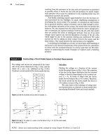
Heating Appliances
In Chapter 9 we calculated the steady-state voltages and cur-
rents in electric circuits driven by sinusoidal sources. In this
chapter we consider power in such circuits. The techniques we
develop are useful for analyzing many of the electrical devices
we encounter daily, because sinusoidal sources are the pre-
dominant means of providing electric power in our homes,
schools, and businesses.
One common class of electrical devices is heaters, which
transform electric energy into thermal energy. Examples include
electric stoves and ovens, toasters, irons, electric water
heaters, space heaters, electric clothes dryers, and hair dryers.
One of the critical design concerns in a heater is power
con-
sumption.
Power is important for two reasons: The more power
a heater uses, the more it costs to operate, and the more heat
it can produce.
Many electric heaters have different power settings corre-
sponding to the amount of heat the device supplies. You may
wonder just how these settings result in different amounts of
heat output. The Practical Perspective example at the end of
this chapter examines the design of a handheld hair dryer

with three operating settings (see the accompanying figure).
You will see how the design provides for three different
power levels, which correspond to three different levels of
heat output.
Heater tube
Fan and motor
Hot air
361
362 Sinusoidal Steady-State Power Calculations
10.1 Instantaneous Power
l
—*"
+
V
Figure 10.1 A
The
black box representation of
a
circuit
used for calculating power.
We begin our investigation of sinusoidal power calculations with the
familiar circuit in Fig.
10.1.
Here, v and
/'
are steady-state sinusoidal signals.
Using the passive sign convention, the power at any instant of time is
VI.
(10.1)
This is instantaneous power. Remember that if the reference direction of

the current is in the direction of the voltage rise, Eq. 10.1 must be written
with a minus sign. Instantaneous power is measured in watts when the
voltage is in volts and the current is in amperes. First, we write expressions
for v and i;
v =
V„,
cos
(cot
+ 0j,),
i —
I„,
cos
{ait
-I- 0,),
(10.2)
(10.3)
where 0,, is the voltage phase angle, and
0-,
is the current phase angle.
We are operating in the sinusoidal steady state, so we may choose any
convenient reference for zero time. Engineers designing systems that
transfer large blocks of power have found it convenient to use a zero time
corresponding to the instant the current is passing through a positive max-
imum. This reference system requires a shift of both the voltage and cur-
rent by
0,
Thus Eqs. 10.2 and 10.3 become
v = V
m
cos (ait + 0,, - 0,),

i =
1,,,
cos
cot.
(10.4)
(10.5)
When we substitute Eqs. 10.4 and 10.5 into Eq.
10.1,
the expression for the
instantaneous power becomes
p =
V
m
I
m
cos
{cot
+ 0
V
-
0j)
cos
cot.
(10.6)
We could use Eq. 10.6 directly to find the average power; however, by sim-
ply applying a couple of trigonometric identities, we can put Eq. 10.6 into
a much more informative form.
We begin with the trigonometric identity
1
1

cos a cos
/3
= — cos (a /3) +-cos(a + /3)
to expand Eq.
10.6;
letting a = cot + 0,, — 0, and
fS
=
cot
gives
p = —— cos (6
V
- 0,) + —r— cos
{loot
+ 0„ - 0,-).
(10.7)
Now use the trigonometric identity
cos (a + /3) = cos a cos
/3 —
sin a sin
(3
See entry
8
in Appendix F.
to expand the second term on the right-hand side of Eq.
10.7,
which gives
y
171*111
/

n
n\ ,
r
111*111
//, ., \ *
p
= ——
cos
(6
V
- 6-)
H
— cos (0,, - 0,) cos
2(ot
V I
- -^- sin (0
V
-
6j)
sin
2u>t.
(10.8)
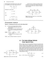
Figure 10.2 depicts a representative relationship among v, i, and p,
based on the assumptions 0.,, - 60° and
6-,
= 0°. You can see that the fre-
quency of the instantaneous power is twice the frequency of the voltage or
current. This observation also follows directly from the second two terms
on the right-hand side of Eq. 10.8. Therefore, the instantaneous power
goes through two complete cycles for every cycle of either the voltage or

the current. Also note that the instantaneous power may be negative for a
portion of each cycle, even if the network between the terminals is passive.
In a completely passive network, negative power implies that energy
stored in the inductors or capacitors is now being extracted. The fact that
the instantaneous power varies with time in the sinusoidal steady-state
operation of a circuit explains why some motor-driven appliances (such as
refrigerators) experience vibration and require resilient motor mountings
to prevent excessive vibration.
We are now ready to use Eq. 10.8 to find the average power at the ter-
minals of the circuit represented by Fig. 10.1 and, at the same time, intro-
duce the concept of reactive power.
Figure 10.2 • Instantaneous power, voltage, and current versus vt for
steady-state sinusoidal operation.
10.2 Average and Reactive Power
We begin by noting that Eq. 10.8 has three terms, which we can rewrite as
follows:
p = P + Pcos2wt - Qs'm2a)t,
(10.9)
364 Sinusoidal Steady-State Power Calculations
where
Average (real) power •
P =
V I
cos (0
V
- e
t
),
(10.10)
Reactive power •

Q =
V I
•sinfo-0,-)-
(10.11)
P is called the average power, and Q is called the reactive power. Average
power is sometimes called real power, because it describes the power in a
circuit that is transformed from electric to nonelectric energy. Although
the two terms are interchangeable, we primarily use the term average
power in this text.
It is easy to see why P is called the average power. The average power
associated with sinusoidal signals is the average of the instantaneous
power over one period, or, in equation form,
>-i
h+T
pdt. (10.12)
where T is the period of the sinusoidal function. The limits on Eq. 10.12
imply that we can initiate the integration process at any convenient time t
{)
but that we must terminate the integration exactly one period later. (We
could integrate over nT periods, where n is an integer, provided we multi-
ply the integral by \fnT.)
We could find the average power by substituting Eq. 10.9 directly into
Eq. 10.12 and then performing the integration. But note that the average
value of/? is given by the first term on the right-hand side of Eq. 10.9,
because the integral of both cos
2cot
and sin
2eot
over one period is zero.
Thus the average power is given in Eq. 10.10.

We can develop a better understanding of all the terms in Eq. 10.9 and
the relationships among them by examining the power in circuits that are
purely resistive, purely inductive, or purely capacitive.
0.01 0.015
Time (s)
0.025
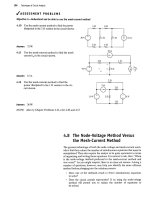
Figure 10.3 • Instantaneous real power and average
power for
a
purely resistive circuit.
Power for Purely Resistive Circuits
If the circuit between the terminals is purely resistive, the voltage and cur-
rent are in phase, which means that $
v
= 0,. Equation 10.9 then reduces to
p = P + P cos
2oot.
(10.13)
The instantaneous power expressed in Eq. 10.13 is referred to as the
instantaneous real power. Figure 10.3 shows a graph of Eq. 10.13 for a
representative purely resistive circuit, assuming
co
= 377 rad/s. By defini-
tion, the average power, P, is the average of/; over one period. Thus it is
easy to see just by looking at the graph that P = 1 for this circuit. Note
from Eq. 10.13 that the instantaneous real power can never be negative,
which is also shown in Fig.
10.3.
In other words, power cannot be extracted
from a purely resistive network. Rather, all the electric energy is dissi-

pated in the form of thermal energy.
Power for Purely Inductive Circuits
If the circuit between the terminals is purely inductive, the voltage and
current are out of phase by precisely
90°.
In particular, the current lags the
voltage by 90° (that is,
6-,
= $
v
-90'); therefore 6,, -
6-,
= +90°. The
expression for the instantaneous power then reduces to
-Q sin
2(ot.
(10.14)
10,2 Average and Reactive Power 365
In a purely inductive circuit, the average power is zero. Therefore no
transformation of energy from electric to nonelectric form takes place.
The instantaneous power at the terminals in a purely inductive circuit is
continually exchanged between the circuit and the source driving the cir-
cuit, at a frequency of
2co.
In other words, when p is positive, energy is
being stored in the magnetic fields associated with the inductive elements,
and when p is negative, energy is being extracted from the magnetic fields.
A measure of the power associated with purely inductive circuits is
the reactive power Q.The name reactive power comes from the character-
ization of an inductor as a reactive element; its impedance is purely reac-

tive.
Note that average power P and reactive power Q carry the same
dimension.To distinguish between average and reactive power, we use the
units watt (W) for average power and var (volt-amp reactive, or VAR) for
reactive power. Figure 10.4 plots the instantaneous power for a represen-
tative purely inductive circuit, assuming
u>
= 311 rad/s and Q = 1 VAR.
Power for Purely Capacitive Circuits
If the circuit between the terminals is purely capacitive, the voltage and
current are precisely 90° out of phase. In this case, the current leads the
voltage by 90° (that is, B
t
= 6
V
+ 90°); thus, 0
V
- 0,- = -90°. The expres-
sion for the instantaneous power then becomes
p = —Qsm2(ot.
(10.15)
Again, the average power is zero, so there is no transformation of energy
from electric to nonelectric form. In a purely capacitive circuit, the power
is continually exchanged between the source driving the circuit and the
electric field associated with the capacitive elements. Figure 10.5 plots the
instantaneous power for a representative purely capacitive circuit, assum-
ing
(o
= 377 rad/s and Q = -1 VAR.
Note that the decision to use the current as the reference leads to Q

being positive for inductors (that
is,
$
v
—
0,
:
= 90° and negative for capac-
itors (that
is,
6
V
- 0, = -90°. Power engineers recognize this difference in
the algebraic sign of Q by saying that inductors demand (or absorb) mag-
netizing vars, and capacitors furnish (or deliver) magnetizing vars.We say
more about this convention later.
o
Q,
Q (VAR)
§ 0 0.005 0.01 0.015 0.02 0.025
| Time (s)
Figure 10.4 • Instantaneous real power, average
power, and reactive power for a purely inductive circuit.
a 0 0.005 0.01 0.015 0.02 0.025
Time (s)
Figure 10.5 • Instantaneous real power and average
power for a purely capacitive circuit.
The Power Factor
The angle 6
V

- 0, plays a role in the computation of both average and
reactive power and is referred to as the power factor angle. The cosine of
this angle is called the power factor, abbreviated pf, and the sine of this
angle is called the reactive factor, abbreviated rf. Thus
pf = cos
(0,,
- 0,),
(10.16) -4 Power factor
rf = sin (0,, - 0/).
(10.17)
Knowing the value of the power factor does not tell you the value of the
power factor angle, because cos (0,, - 0
(
) = cos (0, - 0„). To completely
describe this angle, we use the descriptive phrases lagging power factor and
leading power factor. Lagging power factor implies that current lags volt-
age—hence an inductive load. Leading power factor implies that current
leads voltage—hence a capacitive load. Both the power factor and the reac-
tive factor are convenient quantities to use in describing electrical loads.
Example 10.1 illustrates the interpretation of P and Q on the basis of
a numerical calculation.