Freeland - Molecular Ecology (Wiley, 2005) - Chapter 3 docx
Bạn đang xem bản rút gọn của tài liệu. Xem và tải ngay bản đầy đủ của tài liệu tại đây (445.56 KB, 46 trang )
3
Genetic Analysis of Single
Populations
Why Study Single Populations?
Now that we know how molecular markers can provide us with an almost endless
supply of genetic data, we need to know how these data can be used to address
specific ecological questions. A logical starting point for this is an exploration of
the genetic analyses of single populations, which will be the subject of this chapter.
We will then build on this in Chapter 4 when we start to look at ways to analyse the
genetic relationships among multiple populations. This division between single
and multiple populations is somewhat artificial, as there are ver y few populations
that exist in isolation. Nevertheless, in this chapter we shall be treating populations
as if they are indeed isolated entities, an approach that can be justified in two ways.
First, research programmes are often concerned with single populations, for
example conservation biologists may be interested in the long-term viability of a
particular population, or forestry workers may be concerned with the genetic
diversity of an introduced pest population. Second, we have to be able to
characterize single populations before we can start to compare multiple popula-
tions. But before we start investigating the genetics of populations, we need to
review what exactly we mean by a population.
What is a population?
A population is generally defined as a potentially interbreeding group of
individuals that belong to the same species and live within a restricted geogra-
phical area. In theory this definition may seem fairly straightforward (at least for
sexually reproducing species), but in practice there are a number of reasons why
Molecular Ecology Joanna Freeland
# 2005 John Wiley & Sons, Ltd.
populations are seldom delimited by obvious boundaries. One confounding factor
may be that species live in different groups at different times of the year. This is
true of many bird species that breed in northerly temperate regions and then
migrate further south for the winter, because any one of these overwintering
‘populations’ may comprise birds from several distinct breeding populations.
The situation is even more complex in the migratory common green darner
dragonfly, Anax junius (Figure 3.1). Throughout part of its range, A. junius has two
alternative developmental pathways in which larvae take either 3 or 11 months to
develop into adults (Trottier, 1966). Individuals that develop at different rates will
not be reproductively active at the same time and therefore cannot interbreed. If
developmental times are fixed there would be two distinct A. junius populations
within a single lake or pond, but preliminary genetic data suggest that develop-
ment in this species is an example of phenotypic plasticity (Freeland et al., 2003).
This means that, although some individuals are unable to interbreed within a
particular mating season, their offspring may be able to interbreed in the following
Figure 3.1 A pair of copulating common green darner dragonflies (
Anax junius
). Juvenile
development in this species is phenotypically plastic, depending on the temperature and photoperiod
during the egg and larval stages. Photograph provided by Kelvin Conrad and reproduced with
permission
64
GENETIC ANALYSIS OF SINGLE POPULATIONS
year; therefore, individuals that follow different developmental pathways can still
be part of the same population.
Prolonged diapause (delayed development) also may cause researchers to
underestimate the size or boundaries of a population, because seeds or other
propagules that are in diapause will often be excluded from a census count. Many
plants fall into this category, such as the flowering plant Linanthus parryae that
thrives in the Mojave desert when conditions are favourable. When the environ-
ment becomes unfavourable, seeds can lay dormant for up to 6 years in a seed
bank, waiting for conditions to improve before they germinate (Epling, Lewis and
Ball, 1960). Similarly, the sediment-bound propagules of many species of fresh-
water zooplankton can survive for decades (Hairston, Van Brunt and Kearns, 1995).
Another complication that arises when we are defining populations is that their
geographical boundaries are seldom fixed. Boundaries may be particularly unpre-
dictable if reproduction within a population depends on an intermediate species.
The population limits of a flowering plant, for example, may depend on the
movements of pollinators, which can vary from one year to the next. Populations
of the post-fire wood decay fungus Daldinia loculata, which grows in the wood of
deciduous trees that have been killed by fire, are also influenced by vectors.
Pyrophilous insect species moving between trees can disperse fungal conidia
(clonal propagules that act as male gametes) across varying distances. Genetic
data from a forest site in Sweden suggested that insects sometimes transfer conidia
between trees, thereby increasing the range of potentially interbreeding individuals
beyond a sing le tree (Guidot et al., 2003).
It should be apparent from the preceding examples that population boundaries
are seldom precise, although in a reasonably high proportion of cases they should
correspond more or less to the distribution of potential mates. Biologists often
identify discrete populations at the start of their research programme, if only as a
framework for their sampling design, which often will specify the minimum
number of individuals required from each presumptive population. Nevertheless,
populations should not be treated as clear-cut units, and the boundaries are
sometimes revised after additional ecological or genetic data have been acquired.
Bearing in mind that molecular ecology is primarily concerned with wild
populations, which by their very nature are variable (Box 3.1) and often
unpredictable, we shall start to look at ways in which molecular genetics can
help us to understand the dynamics of single populations.
Box 3.1 Summarizing data
Ecological studies, molecular and otherwise, are often based on measure-
ments of a trait or characteristic that have been taken from multiple
individuals. These data may quantify phenotypic traits, such as wing
lengths in birds, or genotypic traits, such as allele frequencies in different
WHY STUDY SINGLE POPULATIONS 65
populations. Consider the following data set on wing lengths:
Sample 1 Sample 2
23 20
21 26
23 23
24 19
24 27
There are a number of ways in which we can summarize these wing
measurements, including the arithmetic mean, or average, which is
calculated as:
"
XX ¼ Æx
i
=n ð3:1Þ
where x
i
is the value of the variable in the ith specimen, so
"
XX ¼ð23 þ 21 þ23 þ24 þ 24Þ=5 ¼ 23 for population 1; and
"
XX ¼ð20 þ 26 þ 23 þ 19 þ 27Þ=5 ¼ 23 for population 2
In this case both populations have the same average wing length, but this
is telling us nothing about the variation within each population. The
range of measurements (the minimum value subtracted from the max-
imum value, which equals 3 and 8 in samples 1 and 2, respectively), can
give us some idea about the variability of the sample, although a single
unusually large or unusually small measurement can strongly influence
the range without improving our understanding of the variability. An
alternative measure is variance, which reflects the distribution of the data
around the mean. Variance is calculated as:
V ¼
Æ
n
i¼1
ðX
i
À
"
XXÞ
2
=ðn À1Þð3:2Þ
¼½ð23 À23Þ
2
þð21 À23Þ
2
þð23 À 23Þ
2
þð24 À 23Þ
2
þð24 À23Þ
2
=ð5 À1Þ
¼ 1:5 for population 1; and
¼½ð20 À23Þ
2
þð26 À23Þ
2
þð23 À 23Þ
2
þð19 À 23Þ
2
þð27 À23Þ
2
=ð5 À1Þ
¼ 12:5 for population 2
This shows that, although the mean is the same in both samples,
the variation in sample 2 is an order of magnitude higher than that in
66 GENETIC ANALYSIS OF SINGLE POPULATIONS
sample 1. Variance is described in square units and therefore can be quite
difficult to visualize so it is sometimes replaced by its square root, which is
known as the standard deviation (S), calculated as:
S ¼
ffiffiffiffi
V
p
ð3:3Þ
¼
ffiffiffiffiffiffi
1:5
p
¼ 1:225 for population 1; and
¼
ffiffiffiffiffiffiffiffiffi
12:5
p
¼ 3:536 for population 2
Quantifying Genetic Diversity
Genetic diversity is one of the most impor tant attributes of any population.
Environments are constantly changing, and genetic diversity is necessary if
populations are to evolve continuously and adapt to new situations. Further-
more, low genetic diversity t y pically leads to increased levels of inbreeding,
which can reduce the fitness of individuals and populations. An assessment of
genetic diversity is therefore central to population genetics and has extremely
important applications in conservation biology. Many estimates of genetic
diversity are based on either allele frequencies or genoty pe frequencies, and it
is important that we understand the difference between these two measures. We
shall therefore start this section with a detailed look at t he expected relationship
between allele and genotype frequencies when a population is in Hardy
Weinberg equilibrium.
Hardy–Weinberg equilibrium
Under certain conditions, the genotype frequencies within a given population will
follow a predictable pattern. To illustrate this point, we will use the example of the
scarlet tiger moth Panaxia dominula. In this species a one locus/two allele system
generates three alternative wing patterns that vary in the amount of white spotting
on the black forewings and in the amount of black marking on the predominantly
red hindwings. Since these patterns correspond to homozygous dominant,
heterozygous and homozygous recessive genotypes, the allele frequencies at this
locus can be calculated from phenotypic data. We will refer to the two relevant
alleles as A and a. Because this is a diploid species, each individual has two alleles at
this locus. The two homozygote genotypes are therefore AA and aa and the
heterozygote genotype is Aa. Recall from Chapter 2 that allele frequencies
are calculations that tell us how common an allele is within a population. In a
two-allele system such as that which determines the scarlet tiger moth wing
QUANTIFYING GENETIC DIVERSITY 67
genotypes, the frequency of the dominant allele (A) is conventionally referred to as
p, and the frequency of the recessive allele (a) is conventionally referred to as q.
Because there are only two alleles at this locus, pþq¼1.
Genotype frequencies, which refer to the proportions of different genotypes
within a population (in this case AA, Aa and aa), must also add up to 1.0. If we
know the frequencies of the relevant alleles, we can predict the frequency of each
genotype within a population provided that a number of assumptions about that
population are met. These include:
There is random mating within the population (panmixia). This occurs if
mating is equally likely between all possible male female combinations.
No particular genotype is being selected for.
The effects of migration or mutation on allele frequencies are negligible.
The size of the population is effectively infinite.
The alleles segregate following normal Mendelian inheritance.
If these conditions are more or less met, then a population is expected to be in
Hardy Weinberg equilibrium (HWE). The genotype frequencies of such a
population can be calculated from the allele frequencies because the probability
of an individual having an AA genotype depends on how likely it is that one A
allele will unite with another A allele, and under HWE this probability is the
square of the frequency of that allele (p
2
). Similarly, the probability of an
individual having an aa genotype will depend on how likely it is that an a allele
will unite with another a allele, and under HWE this probability is the square of
the frequency of that allele (q
2
). Finally, the probability of two gametes yielding an
Aa individual will depend on how likely it is that either an A allele from the male
parent will unite with an a allele from the female parent (creating an Aa
individual), or that an a allele from the male parent will unite with an A allele
from the female parent (creating an aA individual). Since there are two possible
ways that a heterozygote individual can be created, the probability of this
occurring under HWE is 2pq.
The genotype frequencies in a population that is in HWE can therefore be
expressed as:
p
2
þ 2pq þq
2
¼ 1 ð3:4Þ
The various frequencies of heterozygotes and homozygotes under HWE are shown
in Figure 3.2, and examples are calculated in Box 3.2.
68 GENETIC ANALYSIS OF SINGLE POPULATIONS
Box 3.2 Calculating Hardy–Weinberg equilibrium
Table 3.1 is an actual data set on scarlet tiger moths that was collected by
the geneticist E.B. Ford. The data in Table 3.1 tell us that in this sample
there is a total of 2(1612) ¼ 3224 alleles at this particular locus. Of these,
3076 are A alleles (2938þ138) and 148 are a alleles (138þ10), therefore
the frequency p of the A allele in this population is:
p ¼ 3076=3224 ¼ 0:954
0.0 0.1 0.2 0.3 0.4 0.5 0.6 0.7 0.8 0.9 1.0
Genotype frequency
0.0
0.1
0.2
0.3
0.4
0.5
0.6
0.7
0.8
0.9
1.0
Genotype frequency
0.0
0.1
0.2
0.3
0.4
0.5
0.6
0.7
0.8
0.9
1.0
q
= 1
p
q
2
(aa)
p
2
(AA)
2p q
(Aa)
1.0 0.9 0.8 0.7 0.6 0.5 0.4 0.3 0.2 0.1 0.0
p
= 1
q
Figure 3.2 The combinations of homozygote and heterozygote frequencies that can be found in
populations that are in HWE. Note that the frequency of heterozygotes is at its maximum when
p ¼q ¼
0.5. When the allele frequencies are between 1/3 and 2/3, the genotype with the highest
frequency will be the heterozygote. Adapted from Hartl and Clark (1989)
Table 3.1 Data from a collection of 1612 scarlet tiger moths
No. of Assumed No. of No. of
Phenotype individuals genotype A alleles a alleles
White spotting 1469 AA 1469 Â2 ¼2938
Intermediate 138 Aa 138 138
Little spotting 5 aa 5 Â2 ¼10
QUANTIFYING GENETIC DIVERSITY 69
and the frequency q of the a allele can be calculated as either:
q ¼ 148=3224 ¼ 0:046
or, because p + q = 1, as:
q ¼ 1 À p ¼ 1 À0:954 ¼ 0:046
If we know p and q, then we can calculate the frequencies of AA (p
2
), Aa
(2pq) and aa (q
2
) that would be expected if the population is in HWE as
follows:
p
2
¼ð0:954Þ
2
¼ 0:9101
2pq ¼ 2ð0:954Þð0:046Þ¼0:0878
q
2
¼ð0:046Þ
2
¼ 0:002
We now need to calculate the number of moths in this population
that would have each genotype if this population is in HWE. We can do
this by multiplying the total number of moths (1612) by each genot ype
frequency:
AA ¼ð0:9101Þð1612Þ¼1467
Aa ¼ð0:0878Þð1612Þ¼142
aa ¼ð0:002Þð1612Þ¼3
Therefore the Hardy Weinberg ratio expressed as the number of
individuals with each genotype is 1467:142:3. This is very close to the
actual ratio of genotypes within the population (from Table 3.1) of
1469:138:5.
We can check whet her or not there is a significant difference between
the obser ved and expected genot y pe f requencies by using a chi-squared
(
2
) test. This is based on the difference between the obser ved (O)
number of genotypes and the number that would be expected (E)
under the HWE, and is calculated as:
2
¼ ÆðO ÀEÞ
2
=E ð3:5Þ
The
2
value of the scarlet tiger moth example is:
2
¼ð1469 À 1467Þ
2
=1467 þð138 À142Þ
2
=142 þð5 À3 Þ
2
=3
¼ 0:0027 þ0:11 þ 1:33
¼ 1:44
70 GENETIC ANALYSIS OF SINGLE POPULATIONS
The number of degrees of freedom (d.f.) is determined as 3 (the
number of genotypes) minus 1 (because the total number was used)
minus 1 (the number of alleles), which leaves d.f. ¼ 1. By using a statistical
table, we learn that a
2
value of 1.44, in conjunction with 1 d.f., leaves
us with a probability of P ¼ 0.230. This means that there is no significant
difference between the observed genotype frequencies in the scarlet
tiger moth population and the genotype frequencies that are expected
under the HWE. We would conclude, therefore, that this population is in
HWE.
Despite the fairly rigorous set of criteria that are associated with HWE,
many large, naturally outbreeding populations are in HWE because in these
populations the effects of mutation and selection will be small. There are also
many populations that are not expected to be in HWE, including those that
reproduce asexually. A deviation from HWE may also be an unexpected result, and
when this happens researchers will try to understand why, because this may tell us
something quite interesting about either the locus in question (e.g. natural
selection) or the population in question (e.g. inbreeding). First, however, we
must ensure that an unexpected result is not attributable to human error.
Deviations from HWE may result from improper sampling. The ideal population
sample size is often at least 30 40, although this will depend to some extent on the
variability of the loci that are being characterized. Inadequate sampling will lead to
flawed estimates of allele frequencies and is therefore one reason why conclusions
about HWE may be unreliable.
Another possible source of error is to inadvertently sample from more than one
population. We noted earlier that identifying population boundaries is often
problematic. If genetic data from two or more populations that have different
allele frequencies are combined then a Wahlund effect will be evident, which
means that the proportion of homozygotes will be higher in the aggregrate sample
than it would be if the populations were analysed separately. This could lead us to
conclude erroneously that a population was not in HWE, whereas if the data had
been analysed separately then we may have found two or more populations that
were in HWE. An example of this was found in a study of a diving water beetle
(Hydroporus glabriusculus) that lives in fenland habitats in eastern England. An
allozyme study of apparent populations revealed significant heterozygosity deficits
(Bilton, 1992), but it was only after conducting a detailed study of the beetle’s
ecology that the author of this study realized that each body of water actually
harbours multiple populations that seldom inter breed. This population subdivi-
sion meant that samples pooled from a single water body represented multiple
populations, and therefore the heterozygosity deficits could be explained by the
Wahlund effect.
QUANTIFYING GENETIC DIVERSITY 71
Estimates of genetic diversity
Now that we have a better understanding of allele and genotype frequencies,
we will look at some ways to quantify genetic diversity within populations. One
of the simplest estimates is allelic diversity (often designated A), which is
simply the average number of alleles per locus. In a population that has four
alleles at one locus and six alleles at another locus, A¼ (4þ6)/2 ¼ 5. Although
straightforward, this method is very sensitive to sample size, meaning that the
number of alleles identified will depend in part on how many individuals
are screened. A second measure of genetic diversity is the proportion of
polymor phic loci (often designated P). If a population is screened at ten loci
and six of these are variable, then P ¼ 6/10 ¼ 0.60. This can be of some utility in
studies based on relatively invariant loci such as allozymes, although it also is
sensitive to sample size. Furthermore, it is often a completely uninformative
measure of genetic diversit y in studies based on variable markers such as
microsatellites which tend to be chosen for analysis only if they are polymorphic
and theref ore will often have P values of 1.00 in all populations. A third measure
of genetic diversity that is also influenced by the number of individuals that
are sampled is obser ved heterozygosity (H
o
), which is obtained by dividing
the number of heterozygotes at a par ticular locus by the total number of
individuals sampled. The observed heterozygosity of the scarlet tiger moth based
on the data in Table 3.1 is 138/1612 ¼ 0.085.
Although one or more of the estimates outlined in the preceding paragraph are
often included in studies of genetic diversity, they are generally supplemented with
an alternative measure known as gene diversity (h; Nei, 1973). The advantage of
gene diversity is that it is much less sensitive than the other methods to sampling
effects. Gene diversity is calculated as:
h ¼ 1 À
Æ
m
i¼1
x
i
2
ð3:6Þ
where x
i
is the frequency of allele i,andm is the number of alleles that have
been found at that locus. Note that the only data required for calculating
gene diversity are the allele frequencies within a population. For any given
locus, h represents the probability that two alleles randomly chosen from the
population will be different from one another. In a randomly mating popu-
lation, h is equivalent to the expected heterozygosity (H
e
), and represents the
frequency of heterozygotes that would be expected if a population is in HWE;
for this reason, h is often presented as H
e
.MostcalculationsofH
e
will be based
on multiple loci, in which case H
e
is calculated for each locus and then averaged
over all loci to present a single estimate of diversity for each populat ion (see
Box 3.3).
72 GENETIC ANALYSIS OF SINGLE POPULATIONS
Box 3.3 Calculating
H
e
In the following example, we will use Equation 3.6 to calculate H
e
from
some data that were generated by a study of the southern house mosquito
(Culex quinquefasciatus) in the Ha waiian Islands (Fonseca, LaP ointe and
Fleischer, 2000). This is an intr oduced species that has caused considerable
devastation on the Hawaiian archipelago because it is the vector for avian
malaria. Table 3.2 shows the allele frequencies at one locus calculated from
two populations.
Following Equation 3.6 and using the data from Table 3.2, H
e
from the
Midway population can be calculated as:
H
e
¼ 1 Àð0:250
2
þ 0:200
2
þ 0:550
2
Þ
¼ 1 Àð0:0625 þ 0:04 þ 0:3025Þ
¼ 0:595
Similarly, H
e
from the Kauai population can be calculated as:
H
e
¼ 1 Àð0:022
2
þ 0:333
2
þ 0:333
2
þ 0:311
2
Þ
¼ 1 Àð0:000484 þ 0:111 þ 0:111 þ0:0967Þ
¼ 0:68
In this case, H
e
is higher in Kauai than Midway, which is not surprising
since the former population has a greater number of alleles and also a more
even distribution of allele frequencies than the latter.
Research papers typically report several different calculations of a population’s
genetic diversity, and these often include both H
o
and H
e
. By comparing these two
values, we can determine whether or not the heterozygosity within a population is
Table 3.2 Allele frequency data for one microsatellite locus characterized in two
Hawaiian populations of
C. quinquefasciatus
. Data are from Fonseca, LaPointe and
fleischer. (2000)
Allele frequencies
Microsatellite alleles (bp) Midway population Kauai population
212 0 0.022
216 0.250 0.333
218 0.200 0.333
224 0.550 0.311
QUANTIFYING GENETIC DIVERSITY 73
significantly different from that expected under HWE. If H
o
is lower than H
e
then
we may have to rule out the possibility of null alleles. Although potentially
applicable to a range of markers, this term is used most commonly to describe
microsatellite alleles that do not amplify during PCR. The most common cause of
this is a mutation in one or both of the primer-binding sequences. If only one
allele from a heterozygote is amplified then it will be genotyped erroneously as a
homozygote. When H
o
is significantly less than H
e
we should also be open to the
possibility of a Wahlund effect, which, as noted earlier, will decrease H
o
. If neither
null alleles nor a Wahlund effect have caused an observed heterozygosity deficit
then we may conclude that the population is not in HWE. As noted earlier, this
deviation could result from one or more of a number of factors, including non-
random mating (e.g. inbreeding), natural selection or a small population size.
It can be difficult to determine just what is responsible for disparities between
H
o
and H
e
. In one study, estimates of H
e
and H
o
were obtained for twelve
European populations of the common ash (Fraxinus excelsior) based on micro-
satellite data from five loci. Deviations from HWE were apparent in ten of these
populations, which is an unusual finding in forest tree populations (Morand et al.,
2002). These deviations were caused by H
o
deficits at all five loci (Table 3.3), a
consistent result that was unlikely to be attributable to natural selection acting on
all five putatively neutral loci. Inbreeding also seemed unlikely in this wind-
pollinated species, because long-distance dispersal of pollen should minimize
mating between relatives. A comparison of microsatellite genotypes between
parents and offspring suggested that null alleles were unlikely to be the cause
but, because no plausible explanation for the observed heterozygote deficit has
been found, the authors could not conclusively rule out either null alleles or a
possible Wahlund effect.
Table 3.3 Number of alleles, expected heterozygosity (
H
e
) and observed heterozygosity (
H
o
) for
three populations of the common ash, based on data from five microsatellite loci. In most cases,
H
e
is
significantly larger than
H
o
. Data from Morand
et al
. (2002)
Locus 1 Locus 2 Locus 3 Locus 4 Locus 5
Population 1
No. of alleles 12 13 12 9 16
H
e
0.938 0.888 0.905 0.833 0.937
H
o
0.385 0.895 0.571 0.750 0.737
Population 2
No. of alleles 12 12 12 11 9
H
e
0.938 0.825 0.936 0.892 0.917
H
o
0.462 0.647 0.333 0.526 0.500
Population 3
No. of alleles 16 12 13 12 12
H
e
0.932 0.905 0.859 0.862 0.918
H
o
0.667 0.875 0.750 0.556 0.882
74
GENETIC ANALYSIS OF SINGLE POPULATIONS
Haploid diversity
Gene diversity (h) also can be calculated for haploid data. Estimates of genetic
diversity based on mitochondrial data, for example, often use h as a measure of
haplotype diversity. In this context, h describes the numbers and frequencies
of different mitochondrial haplotypes and is essentially the heterozygosity equi-
valent for haploid loci. However, the haplotype diversity of relatively rapidly
evolving genomes such as animal mtDNA will often approach 1.0 within a
population if a high proportion of individuals have unique haploty pes. It can be
more informative, therefore, to consider the number of nucleotide differences
between any two sequences as opposed to simply determining whether or not
they are different. This can be done by calculating nuc leotide diversit y (;Nei,
1987), which quantifies the mean divergence between sequences. Nucleotide
diversity is calculated as:
¼ Æf
i
f
j
p
ij
ð3:7Þ
where f
i
and f
j
represent the frequencies of the ith and jth haplotypes in the
population, and p
ij
represents the sequence divergence between these haplotypes.
By factoring in both the frequencies and the pairwise divergences of the different
sequences, p calculates the probability that two randomly chosen homologous
nucleotides will be identical.
Choice of marker
When comparing populations, it is important to realize that estimates of genetic
diversity will vary depending on which molecular markers are used. This is
because, as noted in earlier chapters, mutation rates vary both within and between
genomes, and rapidly evolving markers such as microsatellites will generally reflect
higher levels of diversity than more slowly evolving markers such as allozymes.
Furthermore, comparisons between nuclear and organelle genomes may be
influenced by past demographic histories; recall from Chapter 2 that the relatively
small effective population sizes of mtDNA and cpDNA mean that mitochondrial
and chloroplast diversity will be lost more rapidly than nuclear diversity following
either permanent or temporary reductions in population size.
Discrepant estimates of genetic diversity were found in a study that used several
different markers to compare European populations of the common carp (Cypri-
nus carpio) (Kohlmann et al., 2003). According to data from 22 allozyme loci, H
o
¼ 0.066, H
e
¼ 0.062 and A ¼ 1.232. Substantially higher values of H
o
¼ 0.788, H
e
¼ 0.764 and A ¼ 5.75 were obtained from four microsatellite loci. An even greater
difference was found in the mitochondrial genome. Mitochondrial haplotypes
identified using PCR-RFLP revealed haplotype and nucleotide diversity estimates
QUANTIFYING GENETIC DIVERSITY 75
of zero. Genetic diversity in European common carp therefore ranges from non-
existent when estimated from mitochondrial markers to highly variable when
estimated from microsatellite markers. This does not, however, mean that
organelle markers always will be less diverse than nuclear markers. Red pine
(Pinus resinosa) populations in Canada showed no allozyme variation and very
little RAPD variation, but a survey of nine chloroplast microsatellite loci revealed
25 alleles and 23 different haplotypes in 159 individuals (Echt et al., 1998). Table
3.4 gives some other examples of genetic diversity estimates that vary depending
on which markers were used.
Regardless of how variable they are, the ef fective number of loci being
screened will be the same as the actual number only if they are in linkage
equilibrium, which will be true only if they segregate independently of each
other during reproduction. Non-random association of alleles among loci is
known as linkage disequilibrium; this can occur for a number of reasons, the
most common being th e proximity of two loci on a chromosome. When
analysing data from multiple loci it is always necessary to test for linkage
disequilibrium before ruling out the possibility that there are fewer independent
loci for genetic analysis than anticipated. Linkage disequilibrium may also cause
loci to behave in an unexpected manner, for example neutral alleles that are
linked to selected alleles will appear non-neutral and are unlikely to be in HWE
even if the population is large and mating is random.
Table 3.4 Comparisons of within-population variation, measured as
H
e
, based on several different
types of markers. Microsatellite loci often are more variable than either allozyme or dominant markers
Species H
e
Reference
Gray mangrove AFLP: 0.19 Maguire, Peakall and
(Avicennia marina) Microsatellites: 0.78 Saenger (2002)
Russian couch grass RAPD: 0.10 Sun et al. (1998)
(Elymus fibrosus) Allozymes: 0.008
Microsatellites: 0.25
Wild and cultivated AFLP: 0.32 Powell et al. (1996)
soybean (Glycine soja RAPD: 0.31
and G. max) Microsatellites: 0.60
Wild barley AFLP: 0.16 Turpeinen et al. (2003)
(Hordeum spontaneum) Microsatellites: 0.47
Lodgepole pine RAPD: 0.43 Thomas et al. (1999)
(Pinus contorta) Microsatellites: 0.73
Chinese native chickens Allozymes: 0.221 Zhang et al. (2002)
(Gallus gallus domesticus) RAPD: 0.263
Microsatellites: 0.759
Pink ling, a marine fish Allozymes: 0.324 Ward et al. (2001)
(Genypterus blacodes) Microsatellites: 0.823
Roe deer Allozymes: 0.213 Wang and Schreiber (2001)
(Capreolus capreolus) Microsatellites: 0.545
76
GENETIC ANALYSIS OF SINGLE POPULATIONS
What Influences Genetic Diversity?
Genetic diversity is influenced by a multitude of factors and therefore varies
considerably between populations. In this section we shall look at some of the
most important determinants of genetic diversity, including genetic drift, popula-
tion bottlenecks, natural selection and methods of reproduction. While reading
about these, it is important to keep in mind that no process acts in isolation, for
example the rate at which a population recovers from a bottleneck will depend in
part on its reproductive ecology. Furthermore, it is difficult to predict the extent to
which a particular factor will influence genetic diversity because no two popula-
tions are the same. Nevertheless, several factors have a universal relevance to
genetic diversity, and these will comprise the remainder of this chapter.
Genetic drift
Genetic drift is a process that causes a population’s allele frequencies to change
from one generation to the next simply as a result of chance. This happens
because reproductive success within a population is variable, w ith some indi-
viduals producing more offspring than others. As a result, not all alleles will be
reproduced to the same extent, and therefore allele frequencies will fluctuate
from one generation to the next. Because genetic drift alters allele frequencies in
a purely random manner, it results in non-adaptive evolutionary change. The
effects of drift are most profound in small populations where, in the absence of
selection, drift will drive each allele to either fixation or extinction within a
relatively short period of time, and therefore its overall effect is to decrease
genetic diversity. Genetic drift will also have an impact on relatively large
populations but, as we shall see later in this chapter, a correspondingly longer
time period is required before the effects become pronounced. Genetic drift is
an extremely influential force in population genetics and forms the basis of one
of the most important theoretical measures of a population’s genetic structure:
effective population size (N
e
). Because genetic drift and N
e
are inextricably
linked,wewillnowspendsometimelookingathowN
e
differs from censu s
population size (N
c
), how it is linked to genetic drift, and what this ultimately
means for the genetic diversity of populations.
What is effective population size?
A fundamental measure of a population is its size. The importance of population
size cannot be overstated because, as we shall see throughout this text, it can
influence virtually all other aspects of population genetics. From a practical point
of view, relatively large populations are, all else being equal, more likely to survive
WHAT INFLUENCES GENETIC DIVERSITY 77
than small populations. This is why the World Conservation Union (IUCN) uses
population size as a key variable, considering a species to be critically endangered if
it consists of a population that numbers fewer than 50 mature individuals. Taken
in its simplest form, population size refers simply to the number of individuals
that are in a particular population this is the census population size (N
c
). From
the point of view of population genetics, however, a more relevant measure is the
effective population size (N
e
).
The N
e
of a population reflects the rate at which g enetic diversit y will be
lost following genetic drift, and this rate is inversely proportional to a popu-
lation’s N
e
. In an ideal population N
e
¼N
c
, but in reality this is seldom the case.
If an actual population of 500 individuals is losing genetic variation through
drift at a rate that would be found in an ideal population of 100 individuals,
then thi s population would have N
c
¼500 but N
e
¼100, in other words it will
be losing diversity much more rapidly than would be expected in an ideal
population of 500. An N
e
/N
c
ratio of 100/500 ¼ 0.2 would not be c on sidered
unusually low; one review calculated the average ratio of N
e
/N
c
in wild
populations, based on the results of nearly 200 published results, as approxi-
mately 0.1 (Figure 3.3; Frankham, 1995). We will now look at three of the most
common reasons why N
e
is often much smaller than N
c
:unevensexratios,
variation in reproductive success, and fluctuating population size. At the end of
this section we will return to an explicit discussion of the relationship between
N
e
, genetic drift, and genetic diversity.
N
e
/
N
c
01
Number of studies
0
2
4
6
8
10
Figure 3.3 A review of published studies revealed a range of
N
e
/
N
c
values in insects, molluscs, fish,
amphibians, reptiles, birds, mammals and plants. Note that although
N
e
is often much less than
N
c
,itis
a theoretical measurement and under some conditions can be greater than N
c
(data from Frankham,
1995, and references therein)
78
GENETIC ANALYSIS OF SINGLE POPULATIONS
What influences
N
e
?
Sex ratios Unequal sex ratios generally will reduce the N
e
of a population. An
excess of one or the other sex may result from adaptive parental behaviour.
Although the mechanisms behind this are not well understood, there is increasing
evidence for parental manipulation of offspring sex ratios in a number of taxo-
nomic groups, including some bird species, which may be responding to environ-
mental constraints such as a limited food supply (Hasselquist and Kempenaers,
2002). Even if the overall sex ratio in a population is close to 1.0, the sex ratio of
breeding adults may be unequal, and it is the relative proportion of reproductively
successful males and females that ultimately will influence N
e
. In elephant seal
populations, for example, fighting between males for access to harems is fierce.
This intense competition means that within a typical breeding season only a
handful of dominant males in each population will contribute their genes to the
next generation, whereas the majority of females reproduce. This disproportionate
genetic contribution results in an effectively female-biased sex ratio.
The effect of an unequal sex ratio on N
e
is approximately equal to:
N
e
¼ 4ðN
ef
ÞðN
em
Þ=ðN
ef
þ N
em
Þð3:8Þ
where N
ef
is the effective number of breeding females and N
em
is the effective
number of breeding males. The importance of the sex ratio can be illustrated by a
comparison of two hypothetical populations of house wrens (Troglodytes aedon),
which tend to produce an excess of females when conditions are harsh (Albrecht,
2000). Each of these populations has 1000 breeding adults. In the first population,
conditions have been favourable for several years and so the N
ef
of 480 was
comparable to the N
em
of 520. The N
e
therefore would be:
N
e
¼ 4ð480Þð520Þ=ð480 þ520Þ¼998
The second population, however, has been experiencing relatively harsh conditions
for some time. As a result, the N
ef
is 650 but the N
em
is only 350. The N
e
in this
population is:
N
e
¼ 4ð650Þð350Þ=ð650 þ350Þ¼910
In this example, the N
e
/N
c
in the first population, which had almost the same
number of males and females, was 998/1000 ¼0.998. The N
e
/N
c
in the
second population, with its disproportionately large number of females, was
910/1000 ¼ 0.910. Although the N
e
/N
c
ratio was smaller in the second population,
the reduction in N
e
that is attributable to uneven sex ratios was actually relatively
WHAT INFLUENCES GENETIC DIVERSITY 79
low in both of these hypothetical populations compared to what we would find in
many wild populations. According to one survey of multiple taxa, uneven sex
ratios cause effective population sizes to be an average of 36 per cent lower than
census population sizes (Frankham, 1995), although not surprisingly there is
considerable variation both within and among species.
Variation in reproductive success Even if a population had an effective sex ratio
of 1:1, not all individuals will produce the same number of viable offspring, and
this variation in reproductive success (VRS) will also decrease N
e
relative to N
c
.
In some species the effects of this can be pronounced. Genetic and demographic
data were obtained from a 17-year period for a steelhead trout (Oncorhynchus
mykiss) population in Washington State, and variation in reproductive success
was found to be the single most important factor in reducing N
e
(Ardren and
Kapuscinski, 2003). When this trout population is at high density, i.e. when N
c
is
large, females experience increased competition for males, spawning sites and
other resources. The successful competitors will produce large numbers of off-
spring whereas the less successful individuals may fail to reproduce. In other
species, variation in reproductive success may have relatively little influence on N
e
.
The relatively high N
e
/N
c
ratio in balsam fir (Abies balsamea; Figure 3.4) has been
attributed partly to overall high levels of reproductive success in this wind-
pollinated species (Dodd and Silvertown, 2000).
The effects of reproductive variation on N
e
can be quantified if we know the
VRS of a population. Reproductive success reflects the number of offspring that
each individual produces throughout its lifetime and therefore can be determined
from a single breeding season in short-lived species, although individuals with
multiple breeding seasons must be monitored for the requisite number of years.
Long-term monitoring of a population of Darwin’s medium ground finch
(Geospiza fortis) on the Gala
´
pagos archipelago provided an estimated VRS of
7.12 (Grant and Grant, 1992a). The effects of VRS on N
e
can be calculated as
follows:
N
e
¼ð4N
c
À 2Þ=ðVRS þ2Þð3:9Þ
If the census population size of G. fortis is 500 on a particular island, then the
influence of variation in reproductive success on N
e
will be:
N
e
¼½4ð500ÞÀ2=ð7:12 þ 2Þ¼219
Therefore, even if the sex ratio is equal, the variation in the number of chicks that
each individual produces w ill cause N
e
to be substantially smaller than N
c
.
VRS may be highest in clonal species. In the freshwater bryozoan (moss animal)
Cristatella mucedo (Figure 3.5), clonal selection throughout the growing season
means that some clones are eliminated whereas others reproduce so prolifically
80 GENETIC ANALYSIS OF SINGLE POPULATIONS
that the N
c
of a population may be in the tens of thousands by the end of the
growing season (Freeland, Rimmer and Okamura, 2001). Because clonal selection
is decreasing the proportion of unique genotypes throughout the summer (Figure
3.6), the VRS must be substantial, with some clones producing no offspring and
others producing large numbers of young. In the most extreme scenario, some
populations of bryozoans and other clonal taxa may become dominated by a single
clone that experiences all of the reproductive success within that population, and
when this happens the effective population size is virtually one (Freeland, Noble
and Okamura, 2000). If this occurs in a population with a large N
c
, the N
e
/N
c
ratio
will approach zero.
Figure 3.4 Balsam fir (
Abies balsamea
). Wind pollination in this species helps to maintain overall
high levels of reproductive success, and this helps to keep the
N
e
/
N
c
ratios high within populations.
Photograph provided by Mike Dodd and reproduced with permission
WHAT INFLUENCES GENETIC DIVERSITY 81
Figure 3.5 A close-up photograph showing a portion of a colony of the freshwater bryozoan
Cristatella mucedo
. These extended tentacular crowns are approximately 0.8 mm wide and capture
tiny suspended food particles. Photograph provided by Beth Okamura and reproduced with
permission
Relative date
Number of alleles
0
5
10
15
20
25
30
0 25 50 75 100 125 150 200175
Figure 3.6 Linear regression of ln-relative date (sampling date represented as number of days after
1 January) versus total number of alleles in a UK population of the freshwater bryozoan
Cristatella
mucedo
(redrawn from Freeland, Rimmer and Okamura, 2001). Clonal selection has reduced the
genetic diversity of this population throughout the growing season, even though the number of colonies
increased during this time. This leads to a reduction in the
N
e
/
N
c
ratio
82
GENETIC ANALYSIS OF SINGLE POPULATIONS
Fluctuating population size Regardless of a species’ breeding biology, fluctua-
tions in the census population size from one year to the next will have a lasting
effect on N
e
. A sur vey of multiple taxa suggested that fluctuating population sizes
have reduced the N
e
of wild populations by an average of 65 per cent, making this
the most important driver of low N
e
/N
c
ratios (Frankham, 1995). This is because
the long-term effective population size is determined not by the N
e
averaged across
multiple years, but by the harmonic mean of the N
e
(Wright, 1969). The harmonic
mean is the reciprocal of the average of the reciprocals, which means that low
values have a lasting and disproportionate effect on the long-term N
e
. A popula-
tion crash in one year, therefore, may leave a lasting genetic legacy even if a
population subsequently recovers its former abundance. A population crash of this
sort is known as a bottleneck and it may result from a number of different factors,
including environmental disasters, over-hunting or disease.
Because fluctuations in population size have such lasting effects on genetic
diversity, we will take a more detailed look at bottlenecks later in this chapter. For
now, we will limit ourselves to looking at how fluctuating population sizes
influence N
e
, which can be calculated as follows:
N
e
¼ t=½ð1=N
e1
Þþð1=N
e2
Þþð1=N
e3
ÞÁÁÁþð1=N
et
Þ ð3:10Þ
where t is the total number of generations for which data are available, N
e1
is the
effective population size in generation 1, N
e2
is the effective population size in
generation 2, and so on.
The fringed-orchid (Platanthera praeclara) is a globally rare plant that occurs in
patches of tallgrass prairie in Canada. The N
e
of most populations is substantially
reduced by fluctuations in population size from one year to the next. If a
population had a census size of 220, 70, 40 and 200 during each of the past
four years, and we assume that N
e
/N
c
¼1.0, then the effects that these fluctuations
would have had on the N
e
can be calculated as:
N
e
¼ 4=½ð1=220Þþð1=70Þþð1=40Þþð1=200Þ
N
e
¼ 82
Even though this population rebounded from the bottleneck that it experienced
in years 2 and 3, this temporary reduction in N
c
means that the current N
e
/N
c
ratio is only 82/200 ¼ 0.41. Note that we have limited our example to a 4-year
period for the sake of simplicity, although a longer period is needed for an accurate
estimation of N
e
.
So far we have looked at how individual factors sex ratios, VRS, and
fluctuating population sizes can influence N
e
. In each of the preceding sections
we calculated the effects of a single variable on N
e
, but in realit y all of these
variables can simultaneously influence a population’s N
e
. We are highly unlikely to
WHAT INFLUENCES GENETIC DIVERSITY 83
have enough information to calculate individually the reduction in N
e
that is
attributable to each relevant variable. In the next section, therefore, we will move
away from examining the effects of single variables and instead look at how we can
calculate a population’s overall N
e
regardless of which factors have caused the
biggest reduction in N
e
.
Calculating N
e
There are three general approaches for estimating N
e
. The first of these, based on
long-term ecological data, requires accurate census sizes and a thorough under-
standing of a population’s breeding biology, neither or which are available for most
species. A second approach is based on some aspect of a population’s genetic
structure at a sing le point in time, e.g . heterozygosity excess (Pudovkin, Zaykin
and Hedgecock, 1996) or linkage disequilibrium (Hill, 1981). The application of
mutation models to parameters such as these can provide estimates of N
e
,
although this approach is not used widely because it makes many assumptions
about the source of genetic variation and can be influenced strongly by demo-
graphic processes such as immigration (Beaumont, 2003).
The third approach, which is considered by many to be the most reliable,
requires samples from two or more time periods that are separated by at least one
generation. Several different methods can then be used to calculate N
e
from the
variation in allele frequencies over time. At this time, the most widely used method
is based on Nei and Tajima’s (1981) method for calculating the variance of allele
frequency change (F
c
) as follows:
F
c
¼ 1=KÆðx
i
À y
i
Þ=½ðx
i
þ y
i
Þ
2
=ð2 Àx
i
y
i
Þ ð3:11Þ
where K ¼ the total number of alleles and i ¼ the frequency of a particular allele at
times x and y, respectively. This value then can be used to calculate N
e
while
correcting for sample size and N
c
by using the following equation (after Waples,
1989):
N
e
¼ t=2½F
c
À 1=ð2S
0
ÞÀ1=ð2S
t
Þ ð3:12Þ
where t ¼ generation time, S
0
¼ sample size at time zero and S
t
¼ sample size at
time t.
The temporal variance in allele frequencies was used to calculate the N
e
of
crested newt (Triturus cr istatus) populations that were sampled from ponds in
western France. Researchers first were able to obtain an accurate census size of
these populations using a standard mark recapture method. As they were
counted, individuals were marked by removing toes, which then were used as
sources of DNA for deriving genetically based estimates of N
e
. The census
84 GENETIC ANALYSIS OF SINGLE POPULATIONS
population size in one pond was approximately 77 newts in 1989 and 73 newts in
1998. The variance in allele frequencies between 1989 and 1998, based on eight
microsatellite loci, provided an N
e
estimate of approximately 12 and an N
e
/N
c
ratio
of 0.16 (Jehle et al., 2001). Other examples of N
e
/N
c
ratios that have been
calculated from temporal changes in allele frequencies are given in Table 3.5.
Estimating N
e
from the variance in allele frequencies can be logistically
challenging because of the time and expense involved in sampling the same
population in multiple years. O btaining samples from museums is one answer to
this, although museum specimens are a finite resource and not all species will have
sufficient representation. Furthermore, some taxa such as soft-bodied invertebrates
are not amenable to preservation in museums, and in many cases plants will be
underrepresented. Practical limitations may also arise from the availability of
markers; because it is based on allele frequencies, the temporal method ideally
should be done with data from co-dominant loci. Dominant data such as AFLPs
can also be used, although, as noted earlier, accompanying estimates of allele
frequencies will assume Hardy Weinberg equilibrium, which may be unrealistic.
Perhaps the biggest drawback to estimating N
e
from the temporal variance in
allele frequencies is the assumption that all changes in allele frequencies are a result
of genetic drift. This does not allow for the possibility that immigrants from other
populations are introducing new alleles and therefore altering allele frequencies
through a process that is completely separate from genetic drift. As we will see in
the next chapter, most populations receive immigrants with some regularity, and
therefore this assumption is unlikely to be met. This problem has been partially
Table 3.5 Some estimates of
N
e
/
N
c
. In all these examples,
N
e
was calculated using a method based
on the temporal variance in allele frequencies
Species N
e
/N
c
Reference
Steelhead trout (Oncorhynchus mykiss) 0.73 Ardren and Kapuscinski (2003)
Domestic cat (Felis catus) 0.40-0.43 Kaeuffer, Pontier and Perrin
(2004)
Red drum, a marine fish 0.001 Turner, Wares and Gold (2002)
(Sciaenops ocellatus)
Crested newt (Triturus cristatus)
Marbled newt (T. marmoratus) 0.16 Jehle et al. (2001)
0.09
Shining Fungus beetle 0.021 Ingvarsson and Olsson (1997)
(Phalacrus substriatus)
Carrot (Daucus carota) 0.71 Le Clerc et al. (2003)
Grizzly bear (Ursus arctos) 0.27 Miller and Waits (2003)
Apache silverspot butterfly 0.001-0.030 Britten et al. (2003)
(Speyeria nokomis apacheana)
Pacific oyster (Crassostrea gigas) <10
À6
Hedgecock, Chow and Waples
(1992)
Giant toad (Bufo marinus) 0.016-0.008 Easteal and Floyd (1986)
WHAT INFLUENCES GENETIC DIVERSITY 85
addressed by a recently developed maximum likelihood (ML) approach that
estimates N
e
from temporal changes in allele frequencies in a way that partitions
the effects of both immigration and genetic drift (Wang and Whitlock, 2003).
Maximum likelihood is a general term for a statistical method that first specifies
a set of conditions underlying a particular data set, and then determines the
likelihood that these particular conditions would have given rise to the data in
question. In the case of N
e
, conditions may include a particular evolutionary
history of the alleles in question, and maximum likelihood would be used to
calculate the probability that different scenarios would have resulted in the
observed variance in allele frequencies (Berthier et al., 2002). Maximum likelihood
is a powerful approach, although it is computationally demanding and analytically
complex. For these reasons it has avoided the mainstream so far, although its
popularity is increasing as computers become more powerful and software
becomes more user-friendly, and it may soon become the analytical method of
choice for several aspects of molecular ecology including estimates of N
e
.
Wang and Whitlock’s (2003) method is an extremely promising development in
the quest for accurate estimates of N
e
. However, it does require data from a
sufficient number of variable markers to allow the detection of even relatively
small changes in allele frequencies; this may be particularly demanding when N
e
is
relatively large and migration rates are relatively small. In addition, it requires
allele frequency data from both the population under investigation (focal popula-
tion) and the populations from which immigrants may be originating (potential
source populations). Assuming that the latter can be identified, one option is to
pool data from all possible source populations and estimate the extent to which
their collective contribution of migrants to the focal population has influenced the
variance in allele frequencies that might otherwise be attributed entirely to drift.
This method was applied to a metapopulation of newts (Triturus cristatus and
T. marmoratus) in France. The N
e
/N
c
ratios ranged from 0.07 to 0.51 when
researchers assumed that changes in allele frequencies were solely a result of drift,
and were 0.05 0.65 when they allowed for the effects of immigrants (Jehle et al.,
2005). Because it aims to separate the effects that genetic drift and migration have
on changing allele frequencies, this approach marks a significant step forward in
the quantification of N
e
. Although none is perfect, methods for estimating N
e
have
become increasingly refined in recent years, and this trend will undoubtedly
continue because accurate estimates of N
e
are crucial for understanding many
different aspects of population genetics and evolution.
Effective population size, genetic drift and genetic diversity
We started this section by identifying genetic drift as one of the key processes that
influences the genetic diversity of populations. We will now return to that concept
by looking at the specific relationship between N
e
, genetic drift and genetic
86 GENETIC ANALYSIS OF SINGLE POPULATIONS
diversity. The genetic diversity of a population will be reduced whenever an allele
reaches fixation (attains a frequency of 1.0) because, when this occurs, the popu-
lation has only one allele at that particular locus. The probability that a novel
mutation will become fixed in a population as a result of genetic drift is 1/(2N
e
) for
diploid loci, in ohter words it is inversely propor tional to the population’s N
e
(Figure 3.7). Since the rate at which alleles drift to fixation also represents the rate
at which all other alleles at that locus will be lost, 1/(2N
e
) can be considered as the
rate at which genetic variation will be lost within a population as a result of genetic
drift.
The predictable relationship between N
e
and genetic drift means that if we
know the effective size of a population and its current genetic diversity (measured
as expected heterozygosity), and if we assume that the population size remains
essentially constant, we can calculate what the heterozygosity will become after a
given time period as:
H
t
¼½1 À 1=ð2N
e
Þ
t
H
0
ð3:13Þ
where H
t
and H
0
represent heterozygosity at time t and time zero, respectively.
Time intervals refer to generations, not years (although they will of course be the
same if the generation time is 1 year). The predicted heterozygosity at time t is
represented more commonly as a proportion of the heterozygosity at time zero:
H
t
=H
0
¼½1 À 1=ð2N
e
Þ
t
ð3:14Þ
This tells us what proportion of the initial heterozygosity will be remaining after t
generations. We can use this equation to compare the expected changes in hetero-
zygosity in two hypothetical populations of crested newts that have a generation
time of 1 year. The first population lives in a lake and retains an effective popula-
tion size of approximately 200 for a period of 10 years. The second population
inhabits a small pond and has an N
e
of approximately 40 for the same time period.
From Equation 3.14 we can estimate the proportional change in heterozygosity as:
H
t
=H
0
¼½1 À 1=ð2 Â200Þ
10
¼½0:9975
10
¼ 0:975
for the lake population, and as:
H
t
=H
0
¼½1 À 1=ð2 Â40Þ
10
¼½0:9875
10
¼ 0:882
for the pond population. This means that the lake population will lose approxi-
mately 2.5 per cent of its initial heterozygosity in ten generations, whereas the
smaller pond population will lose around 12 per cent of its heterozygosity.
The rate of drift does not depend solely on a population’s N
e
; it is also
influenced by the population sizes of the genome in question (Table 3.6 and
Figure 3.7). Since the population sizes of plastids and mitochondria are effectively
WHAT INFLUENCES GENETIC DIVERSITY 87