Research Techniques in Animal Ecology - Chapter 11 pps
Bạn đang xem bản rút gọn của tài liệu. Xem và tải ngay bản đầy đủ của tài liệu tại đây (400.25 KB, 54 trang )
Chapter 11
Modeling Species Distribution with GIS
Fabio Corsi, Jan de Leeuw, and Andrew Skidmore
From the variety of checklists, atlases, and field guides available around the
world it is easy to understand that distribution ranges are pieces of information
that are seldom absent in a comprehensive description of species. Their uses
range from a better understanding of the species biology, to simple inventory
assessment of a geographic region, to the definition of specific management
actions. In the latter case, knowledge of the area in which a species occurs is
fundamental for the implementation of adequate conservation strategies.
Conservation is concerned mostly with fragmentation or reduction of the dis-
tribution as an indication of population viability (Maurer 1994), given that,
for any species, range dimension is considered to be correlated to population
size (Gaston 1994; Mace 1994).
Unfortunately, animals move and this poses problems in mapping their
occurrence. Traditional methods used to store information on species distri-
butions are generally poor (Stoms and Estes 1993). Distributions have been
described by drawing polygons on a map (the “blotch”) to represent, with
varying approximations, a species’ ranges (Gaston 1991; Miller 1994). The
accuracy of the polygons relies on the empirical knowledge of specialists and
encloses the area in which the species is considered likely to occur, although
the probability level associated with this “likelihood” is seldom specified. A
more sophisticated approach divides the study area into subunits (e.g., admin-
istrative units, equal-size mesh grid), with each subunit associated with infor-
mation on the presence or absence of the species. In this case the distribution
range of a species is defined by the total of all subunits in which presence is
confirmed; however, blank areas are ambiguous as to whether the species is
absent or no records were available (Scott et al. 1993).
390 CORSI, DE LEEUW, AND SKIDMORE
New approaches tend to overcome the concept of distribution range and
move toward one of area of occupancy.
1
This concept is particularly useful for
conservation action and has therefore been included in the new iucnRed List
criteria (iucn1995). In this chapter we outline the basis of identifying distri-
butions that represent a step toward the definition of a real area of occupancy.
For example, imagine a biologist who needs to find zebras. Intuitively, the
odds of finding zebras in Scandinavia are very low, but moving to Kenya
greatly increases the odds. This process is based on very basic assumptions such
as that zebras live in warm places, say, with an average annual temperature of
13–28°C. Obviously our observer won’t expect to find zebras in every place on
Earth that has an average annual temperature of 13–28°C; there are many
other ecological requirements, along with other reasons, such as historical con-
straints (see Morrison et al. 1992 for a review) and species behavioral patterns
(Walters 1992), that contribute to define the distribution of the zebra. Never-
theless, if our biologist extends the same process, taking into account the pre-
ferred ranges of values of various environmental variables, the probability of
finding the species in the areas in which these preferences are simultaneously
satisfied increases.
If the aim of our researcher is to map the areas in which the species is most
likely to be found rather than to find an individual, the entire process can be
seen as a way of describing the species’ presence in terms of correlated envi-
ronmental variables. And if inexpensive and broadly acquired environmental
data (e.g., vegetation index maps derived from satellite data) are used to define
species probability of presence, then maps of species distribution can be pro-
duced quickly and efficiently.
To provide a formal approach to species distribution modeling, the process
can be divided into two phases. The first phase assesses the species’ preferred
ranges of values for the environmental variables taken into account, and the
second identifies all locations in which these preferred ranges of values are ful-
filled. The first phase is generally called habitat suitability index (hsi) analysis,
habitat evaluation procedures (hep) (Williams 1988; Duncan et al. 1995), or,
more generally, species–environment relationship analysis. The second, which
involves the true distribution model, has seen its potential greatly enhanced in
the last 10 years by the increasing use of geographic information systems (
GIS),
which can extrapolate the results of the first phase to large portions of territory.
The power of
GIS resides in its ability to handle large amounts of spatial
data, making analysis of spatial relationships possible. This increases the num-
ber of variables that can be considered in an analysis and the spatial extent to
which the analysis can be carried out (Burrough 1986; Haslett 1990).
Modeling Species Distribution with GIS
391
Thus GIS provides a means for addressing the multidimensional nature of
the species–environment relationship (Shaw and Atkinson 1990) and the need
to integrate large portions of land (eventually the entire biosphere) into the
analysis (Sanderson et al. 1979; Klopatek et al. 1983; Flather and King 1992;
Maurer 1994) to produce robust conservation oriented models.
This chapter is a review of models and methods used in
GIS-based species
distribution models; it is based on a literature review carried out on
GEOBASE
2
with the following keywords: GIS, remote sensing (RS), wildlife, habitat, and dis-
tribution. The 82 papers collected were classified according to the main tool
used (
GIS or RS), the modeling approach, the analysis technique, the discussion
of the assumptions, and the presence of a validation section. At the same time,
information was gathered on the use of the term habitat, the number of vari-
ables used for modeling, and the kind of output produced.
Far from being comprehensive, the review was the starting point for a ten-
tative classification of
GIS distribution models that is presented in this chapter;
at the same time, it allowed us to focus attention on some issues that we con-
sider among the most important for correct use of
GIS in species distribution
modeling. In fact, although it offers powerful tools for spatial analysis,
GIS has
been largely misused and still lacks a clear framework to enable users to exploit
its potential fully.
These issues range from unspecified objectives in the process of model
building to the lack of adequate support for the assumptions underlying the
models themselves. A large part of the chapter is devoted to the problem of val-
idation, which we believe is crucial throughout the process of model building
but is very seldom taken into account.
Before discussing these issues, we address the problem of terminology
inconsistencies, which has a much broader extent in ecology than the specific
realm of species distribution modeling. The problem emerges from our review
and is probably caused, in this context, by misleading use of the same term in
the different disciplines that have come to coexist under the wide umbrella
of
GIS.
Terminology
Multidisciplinary fields of science are very appealing because they bring
together people with different experience and backgrounds whose constructive
exchange of ideas may generate new solutions. In fact, many solutions that
have been successfully developed and used in one field of science may, with
392 CORSI, DE LEEUW, AND SKIDMORE
minor changes, be used in other fields. The very nature of GIS makes it essen-
tial that specialists in different scientific disciplines contribute to the general
effort of setting up and maintaining common data sets.
One drawback is that in the early phases of tool development (such as
GIS),
people who master the new tool tend to become generalists, invading other
fields of science without having the necessary specific background. This may
cause problems both in the solutions provided, which generally tend to be too
simplistic, and in terminology, because the same term or concept can be used
with slightly different meanings in different disciplines. This is the case, for
instance, with use of the concept of scale. For the cartographer, large scale per-
tains to the domain of detailed studies covering small portions of the earth’s
surface (Butler et al. 1986), whereas for the ecologist large scale means an
approach that covers regional or even wider areas (Edwards et al. 1994). Obvi-
ously this derives from the fact that cartographers use scale to mean the ratio
between a unit measure on the map and the corresponding measure on the
earth’s surface, whereas the ecologist uses it in the sense of proportion or
extent. For example, the relationship between the geographic scale and the
extension of ecological studies supplied by Estes and Mooneyhan (1994) high-
lights that large scale in ecology is often associated with small geographic scale:
Site = 1:10,000 or larger
Local = 1:10,000 to 1:50,000
National or regional = 1:50,000 to 1:250,000
Continental = 1:250,000 to 1:1,000,000
Global = 1:1,000,000 or smaller
In ecology it would be better to use the adjectives fine or broad (Levin 1992),
which places the term scale more in the context of its second meaning.
If the confusion arising from the two uses of large scale seems trivial (at least
from the ecologists’ point of view), we believe that the different uses that have
been made of the word habitat give rise to major misunderstandings and thus
need to be clarified (Hall et al. 1997).
Habitat Definitions and Use
The term habitat
3
forms a core concept in wildlife management and the dis-
tribution of plant and animal species. The fact that the actual sense in which it
Modeling Species Distribution with GIS
393
is used is rarely specified suggests that its meaning is taken for granted. How-
ever, Merriam-Webster’s dictionary (1981) provides two different definitions
and Morrison et al. (1992) observed that use of the word habitat remains far
from unambiguous. The latter distinguished two different meanings: one con-
cept that relates to units of land homogeneous with respect to environmental
conditions and a second concept according to which habitat is a property of
species.
Our literature review provided us with a variety of definitions and uses of
the term habitat that are wider than the dichotomy suggested by Morrison et
al. (1992). We arranged these various meanings according to two criteria:
whether the term relates to biota (either species and or communities) or to
land, and whether it relates to Cartesian (e.g., location, such as a position
defined by a northing and easting) or environmental space (e.g., the environ-
mental envelope defined by factors such as precipitation, temperature, and
land cover) (table 11.1).
Although the classification in table 11.1 allows us to partition the different
definitions of habitat we have traced, in reality this partition is rather hazy. For
instance, definitions range from the place where a species lives (Begon et al.
1990; Merriam-Webster 1981; Odum 1971; Krebs 1985), which is a totally
Cartesian space–related concept, to the environment in which it lives (Collin
1988; Moore 1967; Merriam-Webster 1981; Whittaker et al. 1973). In this
last case habitat is seen as a portion of the environmental space. At both
extremes of the range of definitions, the slight differences in the terms used
allows us to define a continuous trend between the Cartesian and the environ-
mental concept, which is further supported considering a few definitions that
combine the Cartesian and the environmental space (Morrison et al. 1992;
Mayhew and Penny 1992). These last authors define habitat as the area that
has specific environmental conditions that allow the survival of a species. Note
that all of these definitions relate habitat to a species and some describe it as a
property of an organism.
With a similar range of definitions, another group relates habitat to both
species and communities. For instance, Zonneveld (1995:26), in accordance
with a Cartesian concept, defined it as “the concrete living place of an organ-
ism or community.” Others relate it to both Cartesian and environmental
space, defining it as the place in which an organism or a community lives,
including the surrounding environmental conditions (Encyclopaedia Britan-
nica 1994; Yapp 1922).
All of the definitions cited so far defined habitat in terms of biota. Zon-
neveld (1995) remarked that the term habitat may be used only when specify-
ing a species (or community). Yet habitat has been used as an attribute of land.
394 CORSI, DE LEEUW, AND SKIDMORE
Table 11.1 Classification Scheme of the Term
Habitat
Biota Land
Species
Species
and Communities
Cartesian space Begon et al. (1990) Zonneveld (1995)
Krebs (1985)
Odum (1971)
Merriam-Webster
(1981)
Cartesian
space and
Morrison et al.
(1992)
Encyclopaedia
Britannica (1994)
Stelfox and
Ironside (1982)
environment Mayhew and
Penny (1992)
Yapp (1922) Kerr (1986)
USFWS
(1980a, 1980b)
Herr and Queen
(1993)
Environment Collin (1988)
Merriam-Webster
(1981)
Whittaker et al.
(1973)
Moore (1967)
The various meanings of habitat are grouped according to whether the term relates to biota (species or
species and communities) or land and whether it relates to Cartesian space, environmental space, or
both.
Riparian habitat, for instance, is a specific environment, with no relation to
biota. Use of habitat in this sense is widespread in the ecological literature (e.g.,
old-forest habitat, Lehmkuhl and Raphael [1993], or woodland habitat,
Begon et al. [1990]). The concept predominates in ecology applied to land
management such as habitat mapping (Stelfox and Ironside 1982; Kerr 1986),
habitat evaluation (USFWS 1980a, 1980b; Herr and Queen 1993), and habi-
tat suitability modeling (USFWS 1981). A similar meaning of habitat is used
in a review of habitat-based methods for biological impact assessment (Atkin-
son 1985). Although it has been used very often in this sense, we were unable
to find a single definition. A closely related concept, the habitat type, which is
used in habitat mapping, has been defined as “an area, delineated by a biolo-
gist, that has consistent abiotic and biotic attributes such as dominant or sub-
Modeling Species Distribution with GIS
395
dominant vegetation” (Jones 1986:23). Daubenmire (1976) noted that this
meaning of habitat type corresponds to the land unit concept (Walker et al.
1986; Zonneveld 1989). In articles dealing with habitat evaluation, the term is
used in a similar sense.
The use of an ambiguous term leads to confusion in communication
between scientists. The ambiguity of habitat is also observed within the same
publication. Lehmkuhl and Raphael (1993), for instance, simultaneously used
“old-forest habitat” and “owl habitat.” Even ecological textbooks are not free
from ambiguity. Begon et al. (1990:853) defined habitat as “the place where a
micro-organism, plant or animal species lives,” suggesting that they consider
habitat a property of a species. However, when outlining the difference
between niche and habitat, they later described habitat in terms of a land unit
(Begon et al. 1990:78): “a woodland habitat for example may provide niches
for warblers, oak trees, spiders and myriad of other species.” Confusion arises
with respect to habitat evaluation as well. When defined as a property of a
species, unsuitable habitat does not exist because habitat is habitable by defi-
nition. In this case some land may be classified as habitat and all of this is suit-
able. When defined as a land property, all land is habitat, whether suitable or
unsuitable, for a specific species.
Why is the term habitat used in these various senses? The word originates
from habitare, to inhabit. According to Merriam-Webster (1981) the term was
originally used in old natural histories as the initial word in the Latin descrip-
tions of species of fauna and flora. The description generally included the envi-
ronment in which the species lives. This leads to the conclusion that habitat
was originally considered a species-specific property. It is interesting to note
that the definitions we traced originated both from ecology and geography,
suggesting that the confusion was not the result of separate developments in
two fields of science.
At some time habitat started to be used as a land-related concept, most
likely in conjunction with habitat mapping. A possible explanation for the
change is given by Kerr (1986), who remarked that mapping habitat
4
individ-
ually for each species would be an impossible job. He argued that a map dis-
playing habitat types and describing the occurrence of species in each type
would be more useful to the land manager. This suggests that the land-related
habitat concept arose because it was considered more convenient to map habi-
tat types rather than the habitat of individual species.
We suggest that there was a second reason for the popularity of habitat type
maps. In general the distribution of species is affected by more than one envi-
ronmental factor. Until a decade ago it was virtually impossible to display
396 CORSI, DE LEEUW, AND SKIDMORE
more than one environmental factor on a single map. The habitat type,
defined as a mappable unit of land “homogeneous” with respect to vegetation
and environmental factors, circumvented this problem and was the basis of the
land system (land concept) maps developed in the 1980s (Walker et al. 1986;
Zonneveld 1989). However, it is based on the assumption that environmental
factors show an interdependent change throughout the landscape and that the
environmental factors are constant within the “homogeneous” area. Thus to a
certain extent the land unit meaning of the term habitat arose as a way to over-
come operational difficulties in species distribution mapping. Nevertheless,
given that the variation of one environmental factor affecting the distribution
of a species often tends to be independent of the other environmental factors,
homogeneity is seldom the case, so there is seldom a true relationship between
species and habitat types.
The advent of
GIS has made it possible to store the variation of environ-
mental factors independently and subsequently integrate these independent
environmental surfaces into a map displaying the suitability of land as a habi-
tat for a specific species.
The first examples of such
GIS-based habitat mapping were published in the
second half of the 1980s (e.g., Hodgson et al. 1988). Since then there has been
a steady increase of the number of
GIS-based habitat models (figure 11.1). The
increase illustrates a move away from the general habitat-type mapping appli-
cable for multiple species toward more realistic species-specific habitat maps.
At the same time, the habitat type loses its usefulness because of the
decreasing need to classify land in homogeneous categories. In other words,
species-specific habitat mapping is increasingly incorporating independent
environmental databases processed using information on the preferences of
the species concerned. In view of the anticipated move toward species-specific
habitat models, we prefer to use the original species-related concept of habitat
instead of a land-related concept; to avoid confusion, in this chapter we will
use the terms species–environment relationships and ecological requirements in-
stead of the terms species habitat and habitat requirements.
General Structure of GIS-Based Models
The rationale behind the GIS approach to species distribution modeling is
straightforward: the database contains a large number of data sets (layers), each
of which describes the distribution of a given measurable and mappable envi-
ronmental variable. The ecological requirements of the species are defined
Modeling Species Distribution with GIS
397
Figure 11.1 Percentage of the papers dealing with habitat modeling using no spatial information,
RS, GIS, and a combination of RS and GIS for three periods (1980–1985, 1986–1991, and 1992–1996).
according to the available layers. The combination of these layers and the sub-
sequent identification of the areas that meet the species’ requirements identify
the species’ distribution range, either actual (if there is evidence of presence) or
potential (if the species has never been observed in that area).
This basic scheme can be implemented using different approaches. A few
classifications based on different criteria have been attempted. For example,
Stoms et al. (1992) classified models based on the conceptual method used to
define the species–environment relationship, whereas Norton and Possingham
(1993) based their classification on the result of the model and its applicabil-
ity for conservation. Accordingly, Stoms et al. (1992) classified
GIS species dis-
tribution models into two main groups—deductive and inductive—whereas
Norton and Possingham (1993) gave a more extensive categorization of mod-
eling approaches.
We have tried to define logical frameworks that can be used to classify
species distribution models based on the major steps that must be followed to
build them. To this end, we find the deductive–inductive categorization the
most suitable starting point because it focuses attention on the definition of
the species–environment relationship, which is the key point for the imple-
mentation of distribution models.
398 CORSI, DE LEEUW, AND SKIDMORE
The deductive approach uses known species’ ecological requirements to
extrapolate suitable areas from the environmental variable layers available in
the
GIS database. In fact, analysis of the species–environment relationship is
relegated to the synthesizing capabilities and wide experience of one or more
specialists who decide, to the best of their knowledge, which environmental
conditions are the most favorable for the existence of the species. Once the
preferences are identified, generally some sort of logical (Breininger et al.
1991; Jensen et al. 1992) or arithmetic map overlay operation (Donovan et al.
1987; Congalton et al. 1993) is used to merge the different
GIS environmental
layers to yield the combined effect of all environmental variables.
When the species–environment relationships are not known a priori, the
inductive approach is used to derive the ecological requirements of the species
from locations in which the species occurs. A species’ ecological signature can
be derived from the characterization of these locations. Then, with a process
that is very similar to the one used in deductive modeling but is generally more
objectively driven by the type of analysis used to derive the signature, it is used
to extrapolate the distribution model (Pereira and Itami 1991; Aspinall and
Matthews 1994).
In figure 11.2 we summarize the data flow of
GIS-based species distribution
models for both the deductive and the inductive approaches. Whereas in the
deductive approach
GIS data layers enter the analysis only to create the distri-
bution model, in the inductive approach they are used both to extrapolate the
species–environment relationship and the distribution model. Along with the
data flow, the steps that need validation are also evidenced in the figure. Vali-
dation is addressed in more detail later in this chapter, but it is interesting to
note here that validation procedures are needed at many different stages in the
flow diagram.
Both inductive and deductive models can be further classified according to
the kind of analysis performed to derive the species–environment relationship.
Essentially these can be subdivided into two main categories: the descriptive
and the analytical. Models pertaining to the first category use either the spe-
cialists’ a priori knowledge (deductive–descriptive) or the simple overlay of
known location of the species with the associated environmental variable lay-
ers (inductive–descriptive) to define the species–environment relationship.
Descriptive models generally are based on very few environmental variable lay-
ers, most often just a single layer. They tend to describe presence and absence
in a deterministic way; each value or class of the environmental variable is asso-
ciated with presence or with absence (e.g., the species is known to live in
savanna with an annual mean temperature of 15–20°C, so savanna polygons
Modeling Species Distribution with GIS
399
Figure 11.2 General data flow of the two main categories of GIS species distribution models identi-
fied in this chapter.
falling within the adequate temperature range are to be included as suitable
environments). No attempt is made to define confidence intervals to the indi-
vidual estimate, nor is any information provided on the relative importance of
one variable over another (e.g., vegetation types vs. temperature). Moreover,
no estimate of the degree of association or its variability is provided with the
relationship.
On the other hand, models that fall into the analytical group introduce
variability in the sense that advice from different specialists is combined to
define species–environment relationships, thus introducing variability in
terms of different opinions of the experts (deductive–analytical), or that the
species observation data are analyzed in a way that takes into account the range
of acceptability of all environmental variables measured, their confidence lim-
its, and their correlation. Both the deductive–analytical and the inductive–
analytical approaches tend to estimate the relative importance of the different
environmental layers considered in the analysis, thus moving toward an objec-
tive combination of environmental variable layers.
Examples of deductive–analytical models are based on techniques such as
multi-criteria decision-making (
MCDM) (Pereira and Duckstein 1993), Delphi
(Crance 1987), and nominal group technique (NGT) (Allen et al. 1987).
Generally speaking, these techniques use the advice of more than one special-
400 CORSI, DE LEEUW, AND SKIDMORE
ist as independent estimates of the “true” species–environment relationship
and evaluate its variability based on these estimates.
Inductive–analytical techniques rely on samples of locations that are ana-
lyzed with some sort of statistical procedure. Different techniques have been
used, including generalized linear models (
GLMs; McCullagh and Nelder 1988;
for applications see Akçakaya et al. 1995; Bozek and Rahel 1992; Pausas et al.
1995; Pearce et al. 1994; Pereira and Itami 1991; Thomasma et al. 1991; Van
Apeldoorn et al. 1994), Bayes theorem approach (Aspinall 1992; Aspinall and
Matthews 1994; Pereira and Itami 1991; Skidmore 1989a), classification trees
(Walker 1990; Walker and Moore 1988; Skidmore et al. 1996), and multi-
variate statistical methods such as discriminant analysis (Dubuc et al. 1990;
Flather and King 1992; Haworth and Thompson 1990; Livingston et al.
1990; Verbyla and Litvaitis 1989), discriminant barycentric analysis (Genard
and Lescourret, 1992), principal component analysis (
PCA) (Lehmkuhl and
Raphael 1993; Picozzi et al. 1992; Ross et al. 1993), cluster analysis (Hodgson
et al. 1987), and Mahalanobis distance (Clark et al. 1993; Knick and Dyer
1997; Corsi et al. 1999).
Models that use simple univariate statistics, such as
ANOVA, Pearson rank
correlation, and Bonferroni, pertain to a different subgroup because these
analyses do not generally allow for definition of the relative importance of the
environmental variables.
Further differences should be outlined for models that rely on the interpo-
lation of density or census estimates to extrapolate distribution patterns.
Although we have included these models in the inductive–analytical group,
the geostatistical approach (Steffens 1992) on which they are generally based
suggests putting them into a slightly different subgroup.
Finally, another means of classifying
GIS distribution models can be based
on their outputs. Essentially, these can be distinguished as categorical–discrete
models and probabilistic–continuous models. Most often the products of the
first type of models are polygon maps in which each polygon is classified accord-
ing to a presence–absence criterion or a nominal category (e.g., frequent, scarce,
absent). The products of the second type of model are continuous surfaces of
an index that describes species presence in terms of the relative importance of
any given location with respect to all the others. Indices that have been used are
the suitability index (Akçakaya et al. 1995; Pereira and Itami 1991), probabil-
ity of presence (Agee et al. 1989; Skidmore 1989a; Aspinall 1992; Clark et al.
1993; Walker 1990), ecological distances from “optimum” conditions (Corsi et
al. 1999), and species densities (Palmeirin 1988; Steffens 1992). All these
indices can be mapped as a continuous surface throughout the species range.
Modeling Species Distribution with GIS
401
Generally, discrete models are built associating the presence of a species to
polygons of land unit types (e.g., vegetation categories), most often with a
deductive approach; in fact, transferring into the realm of
GIS, the traditional
way of producing distribution maps is based on a similar but more arbitrary
partitioning of the study area (e.g., administrative boundaries, regular grids;
see also “Habitat Definitions and Use”). There are also some examples of
binary classifications of continuous environmental variables (e.g., slope,
aspect, elevation) using statistical techniques such as logistic regression (Pereira
and Itami 1991) or discriminant analysis (Corsi et al. 1999). Categorical–dis-
crete models do not account for species mobility and tend to give a static
description of species distribution. Nevertheless, this approach can be used to
address the problem of defining areas of occupancy (Gaston 1991) and thus
can be used successfully for problems of land management and administra-
tion. On the other hand, probabilistic models can describe part of the stochas-
ticity typical of locating an individual of a species and can be used to address
problems of corridor design and metapopulation modeling (Akçakaya 1993),
introducing the geographic dimension in the analysis of species viability.
LITERATURE REVIEW
Table 11.2 indicates the results of our bibliographic review. Papers are classi-
fied according to the categories described in the previous paragraph.
We have considered
GIS and RS as two different views of the same tool, the
former being more devoted to spatial correlation analysis and the later more
concerned with basic data production. In fact, the two families of software
tools share many basic functions and are evolving toward integration into a
single system. It should be noted that the review includes not only papers that
use
GIS or RS but also some that deal with HSI, HEP and general assessment of
species’ ecological requirements. The papers in this last group do not generally
represent examples of spatial models (Scott et al. 1993), in the sense that their
products are not distribution maps, but they have been included because they
are considered to be just a few steps away from a real distribution model. In
fact, they describe the ecological requirements of the species in terms of map-
pable environmental conditions.
Most of the papers that use the deductive approach consider the a priori
knowledge sufficient to define the ecological requirements of the species under
investigation. This is especially true of papers that model distribution on the
basis of interpretation of remotely sensed data; in fact, 15 out of 16 papers per-
taining to the deductive group that used remotely sensed data to model species
402 CORSI, DE LEEUW, AND SKIDMORE
Table 11.2 Classification of Reviewed Papers
Deductive
Descriptive
GIS GIS
and RS
RS
Non-
spatial
GIS GIS
and RS
RS
Non-
spatial
9 8 7 8 32 3 1 0 0 4 36
Analytical
GIS GIS and
RS
RS
Non-
spatial
GIS GIS
and RS
RS
Non-
spatial
301 4 81444163846
40 42
Papers are classified according to the approach used to define the species–environment relationship and
whether their approach was descriptive or analytical. Further subtopics indicate whether the author
considers the research to pertain to the domain of RS, GIS, or both. Nonspatial is used for papers that do
not contain an explicit distribution model but define species–environment relationship in terms of
mappable variables.
Inductive
distributions fall within the descriptive group. In these papers, image classifi-
cation techniques tend to receive more emphasis, whereas the ecological appli-
cation is most often seen as an excuse to apply a specific classification algorithm.
The time trend of the papers published shows rather stable use of
RS tech-
nology and increasing use of
GIS. Up to 1986, no paper makes explicit reference
to the term
GIS, even though some of the papers dealing with the use of RS do
use raster
GIS-style overlay procedures to define their distribution models (e.g.,
Lyon 1983) and others do use a spatial approach but do not mention
GIS (e.g.,
Mead et al. 1981).
Little is generally said about model assumptions. Of the 82 papers
reviewed, only 21 discuss their assumptions. Those that do generally limit
their discussion to the statistical assumptions of the technique used to perform
the analysis. Very few deal with the biological and ecological assumptions and
tend to take them for granted. When dealing with ecological modeling, we
need to take into account both biological and methodological assumptions,
along with some general assumptions that may limit the applicability of the
results produced (Starfield 1997).
Validation, a step that is evidenced at different levels in the data flow dia-
gram (figure 11.2), is generally limited to the accuracy of the result of the
analysis (e.g., distribution map); nothing is said about the accuracy of the orig-
inal data sets (e.g.,
GIS data layers, observation locations) and no consideration
is given to issues such as error propagation in
GIS overlay (Burrough 1986).
Only 15 papers validate of the accuracy of their results based on an inde-
Modeling Species Distribution with GIS
403
pendent estimate of the distribution (either through comparison with an inde-
pendent set of observations or through comparison with the known distribu-
tion of the species); interestingly, 50 percent of these papers are based on the de-
ductive approach. In fact, it should be noted that because observation data sets
are the most expensive data to be collected within the general framework of set-
ting up a
GIS species distribution model, the deductive approach is the most cost-
effective if seen from the validation point of view. In fact, to avoid bias, a model
developed with an inductive approach cannot be validated using the same data
set used to derive the species–environment relationship. Thus validation can be
performed either with a second, independent data set or by dividing the origi-
nal data set into two subsets, one of which is used to derive species–environment
relationships and the other to validate the resulting model.
Finally, it is interesting to note that the multidimensional power of
GIS is still
not backed up by adequate quantity and quality of geographic data sets (Stoms
et al. 1992). This is reflected in the number of environmental variables used in
analysis. In the papers reviewed, the average is just below 4.8, and only 9 out of
82 analyze more than 9 environmental variables, whereas 23 papers base their
distribution models on only one environmental variable, generally vegetation.
Modeling Issues
Based on the results of the literature review, we have identified five major issues
that must be addressed to allow a sound
GIS modeling of species distributions.
These range from uncertainties in the objectives of the research to the lack of
adequate support for the assumptions underlying the implementation of
GIS
models. A problem that is gaining awareness is that of scale, in both time and
space, but it still suffers from inadequate tools.
Slightly different is the issue of data availability, which is rarely addressable
by the biologist concerned with species distribution modeling but limits the
type of models that can be developed.
Finally, a review of sources of errors and ways of estimating the accuracy of
a
GIS model addresses the problem of validation.
CLEAR OBJECTIVES
When setting up an ecological model, the very first step to be considered is
clear statement of the model’s objective (Starfield 1997). There is great confu-
sion about the objectives of many published papers. This may caused by
overqualification of the tool, in the sense that use of the tool becomes the
404 CORSI, DE LEEUW, AND SKIDMORE
objective of the paper, or by uncertainty in defining the model’s goals, along
with coexisting purposes of predicting or understanding (Bunnell 1989). For
instance, most of the papers based on the inductive approach deal with the def-
inition of a species–environment relationship without specifying whether they
intend to analyze the relationship of cause and effect or just use the relation-
ship as a functional description of the effect. In the first case, the goal would be
to evidence the limiting factors that are related to the species’ biological needs
and that drive the distribution process; in the second, it would be the simple
use of correlated variables whose distribution is functional to the description
of the species’ distribution.
Basically, we can summarize species needs as food, shelter, and adequate
reproduction sites (Flather et al. 1992; Pausas et al. 1995). When using the dis-
tribution of an environmental variable to describe the species’ distribution we
implicitly assume that there is a correlation between these basic needs and the
environmental variables used. This correlation can be causal; that is, it
describes the species’ basic needs. In such cases we can identify a function that
within a reasonable range of values associates each value of the environmental
variable to a measure of the fulfillment of the species’ basic needs (e.g., repro-
ductive success). But it can also be a functional description; that is, we don’t
really know why some ranges of values of the environmental variable are pre-
ferred by the species but we observe that the species tends to occur more fre-
quently within those ranges. The variable might influence all the species’ basic
needs simultaneously or be correlated to another variable that describes one of
the species’ needs.
Generally speaking, the quantity and quality of the locational data and the
GIS layers used in analyses are not sufficient to assess cause–effect relationships
that determine the species’ distribution. Furthermore, cause–effect relation-
ships spring from the interactions of biophysical factors that range through
different time and space scales (Walters 1992); few papers take scale depen-
dency into account in their analysis. Moreover in this kind of analysis causal
effects can be hidden by independent interfering variables (Piersma et al.
1993) or by the unaccounted stochasticity of natural events such as weather
fluctuations, disturbance, and population dynamics (Stoms et al. 1992) and
should be assessed in controlled environments.
We believe such uncertainties could be addressed by defining the overall goal
as the assessment of the relationship that best describe the species distribution.
In other words, even if the causal understanding of a relationship is not clear,
whenever the species–environment relationship is able to describe the distribu-
tion of a species satisfactorily, the overall goal is achieved (Twery et al. 1991).
Modeling Species Distribution with GIS
405
Obviously the approach just described has some drawbacks. Without an
adequate description of the cause–effect relationship between the species and
environmental variables, models lose in transferability, in both space and time,
and this limits their predictive capabilities (Levin 1992).
ASSUMPTIONS
All models analyzed extrapolate their results to an entire study area on the
assumption of space independence of the phenomenon observed at a given
place. That is, in the case of both a deductive and an inductive approach, the
species–environment relationship is built on evidence that a certain species
occurs somewhere and that we know the values of the environmental variables
at those locations. Obviously we know only that a species occurs at locations
where it has been observed, only part of these locations have measurements of
the environmental variables, and usually these measurements are collected only
for the limited time range during which the investigation was carried out. Thus,
when building distribution models, evidence collected in a portion of the range
is extrapolated to the entire range of occurrence of a species. In order to do so,
it is assumed that the species–environment relationship used to build the model
is invariant in space and time. Most of the time this is not the case, especially
for species with a wide range and for generalist species. In fact, the higher the
variance of the species–environment relationship, the higher the number of
locations required to provide an adequate ecological profile for the species.
Second, it is generally implicitly assumed that variables that are not
included in the analysis have a neutral effect on the results of the model. That
is, we need to assume either that the species’ ecological response to these envi-
ronmental variable is constant or that the response is highly correlated with the
other variables included.
Even though both of these general assumptions are very difficult to test, we
believe that they should be discussed on a case-by-case basis because the result
of their violation is species-specific. Errors may be negligible in certain cases
but can introduce major interpretation problems in other cases.
Biological assumptions
Biological assumptions are direct consequences of the general assumptions dis-
cussed in the previous paragraph. We nevertheless believe that they are proba-
bly the most critical, but have received minimal attention in the literature.
The first assumption, which follows from the general assumption of space
406 CORSI, DE LEEUW, AND SKIDMORE
and time independence, states that observations reflect distribution. In other
words, information on absence can be derived from observation data (Rexstad
et al. 1988; Clark et al. 1993), which is obviously seldom the case. In fact, any
time we have a record for a species we can be sure that the species (at least occa-
sionally) occurs at that location. In contrast, if there is no observation for a
species, we can only assume that we have a record of absence if there is no bias
in our sampling scheme and that we have conducted our observations over a
sufficiently long period. Even then we have no way of evaluating the random
effects that are intrinsic in observing animals.
These assumptions can have statistical relevance in dealing with induc-
tive–analytical approaches, but must hold true also for the deductive models.
If there is a constant bias in the visibility of a species’ individuals, for instance
because part of their range is less accessible than others to researchers and thus
cannot be as carefully investigated, the species–environment relationship re-
flects this bias. For instance, observation data are often gathered through sight-
ings carried out by volunteers (Stoms et al. 1992; Hausser 1995), which do not
follow a predefined (e.g., random) sampling scheme. Habitat cover may limit
observations to areas where the species is visible (Agee et al. 1989). This may
create an artificial response curve that associates a positive relationship to the
values of the environmental variables measured in the locations where the
species is more visible and a negative one in the ones measured in areas were
the species has been less investigated. In such cases, we would end up mapping
the areas where the species and the observers are most likely to meet, not the
true distribution of the species.
This example is tailored to inductive–analytical models but can easily be
extended to deductive ones, both descriptive and analytical, considering that
the deductive approach is based on the a priori knowledge of specialists who
rely on series of observations to gain experience and define the species–envi-
ronment relationship. Again, these observations can suffer from accessibility
or visibility biases.
A further assumption is that observations reflect the environmental selec-
tion of the species. Obviously this is not always true; for example, occurrences
of migrant or vagrant individuals whose presence in a given location is occa-
sional may be considered among observations. An extreme case is represented
by locust swarms blown into the middle of the desert by strong winds. Clearly,
their presence does not reflect any ecological preference. Nevertheless, if we
consider only the observation per se, we would conclude that high densities of
locusts are found in the desert and that locusts do prefer (with all the limita-
tions that this term carries along in such an analysis) desert environments.
Modeling Species Distribution with GIS
407
Obviously the strong wind of the example should be regarded as a stochastic
event and thus be treated as an outlier in the definition of a possible
GIS distri-
bution model. In other words, observations should be analyzed for their con-
tent of unconstrained selection by the species.
We will see, when dealing with the issues of scale, that
GIS distribution
models tend to describe only the deterministic components that drive a
species’ distribution pattern, so stochastic events must be either averaged on
the long term or eliminated as outliers. When observations are carried out for
a limited time and the biology of the species under investigation is scarcely
known, this problem can become increasingly important because the identifi-
cation of outliers will be virtually impossible.
Statistical assumptions
Most of the statistical techniques used to define species–environment relation-
ships rely on the identification of two observation sets: one that identifies loca-
tions in which the species is present and one in which it is absent. Even though
this cannot be identified properly as a statistical assumption, it is probably the
most important factor limiting the applicability of the statistical techniques
that rely on the two groups of observations.
The most common way to define the two subsets is to compare locations
of known presence with a random sample of locations not pertaining to the
previous set. Obviously some of the random locations can represent a suitable
environment for the species, thus introducing, for that particular environ-
ment, a bias that underestimates the species–environment association.
To overcome this problem, data sets can be screened for outliers (Jongman
et al. 1995), using for instance a scatter plot of the variables taken two by two.
Once an outlier is identified, it can be checked to identify possible reasons for
the absence of the species and, if necessary, removed from the analysis. Similar
results can be achieved through analyses such as decision trees, where addi-
tional rules can be introduced to predict outliers (Walker 1990; Skidmore et
al. 1996).
Another way to get around the problem is to eliminate the absence sub-
group. Skidmore et al. (1996), for example, used both the
BIOCLIM approach
and the supervised nonparametric classifier, which use only observation sites
to derive distribution patterns. The same result can also be achieved by using
distance (or similarity) measures from the environmental characteristics of
locations in which the species has been observed. A measure of distance that
seems particularly promising for this application is the Mahalanobis distance
408 CORSI, DE LEEUW, AND SKIDMORE
(Clark et al. 1993; Knick and Dyer 1997). It has many interesting properties
as compared to other measures of similarity and dissimilarity, the most appeal-
ing of which is that it takes into account not only the mean values of the envi-
ronmental variables measured at observation sites, but also their variance and
covariance. Thus the Mahalanobis distance reflects the fact that variables with
identical means may have a different range of acceptability and eliminates the
problem that the use of correlated variables can have in the analysis.
Along with the identification of presence–absence data sets, each statistical
method has some specific assumption that must be satisfied for correct appli-
cation of the technique. For example, nonparametric statistical tests may
assume that a distribution is symmetric, whereas a parametric test may assume
that the test data are normally distributed. We will not discuss further the
assumptions of the different statistical methods because they are beyond the
scope of this chapter; we refer the reader to more specific books and journal
articles on statistical methods.
SPATIAL AND TEMPORAL SCALE
Scale is a central concept in developing species distribution models with GIS.As
mentioned earlier in this chapter, this concept is common to both geography
and ecology, the two main disciplines involved in the development of
GIS
species distribution models. The concept of scale evolves from the representa-
tion of the earth surface on maps and is the ratio of map distance to ground
distance. Scale determines the following characteristics of a map (Butler et al.
1986): the amount of data or detail that can be shown, the extent of the infor-
mation shown, and the degree and nature of the generalization carried out.
This group of characteristics determines the quality of the layers derived,
that is, the quality of the environmental variables stored in the
GIS database and
the type of species–environment relationship that can be investigated (Bailey
1988; Levin 1992; Gaston 1994) using the capabilities of the
GIS.
The scale of the analysis influences the type of assumptions that need to
hold true for sound modeling. To clarify this concept, we need to consider that
species distribution is the result of both deterministic and stochastic events.
The former tend to be described in terms of the coexistence of a series of envi-
ronmental factors related to the biological requirements of the species, whereas
stochastic processes are regarded as disturbances caused by unpredictable or
unaccountable events (Stoms et al. 1992). Generally distribution models are
built on deterministic events and are averaged over wide spatial and temporal
ranges to minimize the error related to the unaccounted stochasticity.
Modeling Species Distribution with GIS
409
As we have seen, GIS distribution models rely on species–environment rela-
tionships to extrapolate distribution patterns based on the known distribution
of the environmental variables. We have also seen that the relationships reflect
the biological needs of the species. The extent to which we need to coarsen our
temporal and spatial scales depends on the stochastic events that must be min-
imized, which in turn depend essentially on the dynamics of the species under
investigation. To this extent, it is important to note that major population
dynamics events happen on different scales in both time and space. In figure
11.3 (modified from Wallin et al. 1992) the two axes indicate the increasing
temporal and spatial scale at which population dynamics events happen. In
accordance with the hypothesis formulated by other authors (O’Neill et al.
1986; Noss 1992), the figure shows a positive correlation between space and
time scales; that is, events that happen on a broader spatial scale are slower and
thus take more time.
As a tool for distribution modeling this graph can be of great help in defin-
ing scale thresholds toward both a minimum and a maximum scale for an
analysis. For instance, when considering cause–effect species–environment
relationships the processes involved (e.g., feeding behavior) must be analyzed
at an adequate scale (e.g., in our example, very detailed scale both in time and
space). On the other hand, if we need to overcome the stochasticity introduced
in our observation scheme by, for instance, individual foraging behavior we
must average our results on a coarser scale in both time and space.
Thus, in
GIS distribution models, both temporal and spatial scales are gen-
erally broadened so that stochastic events can average to a null component and
thus be ignored. For instance, the stochasticity associated with the individual
selection of a particular site, which greatly influences the distribution at a local
scale, is overcome when dealing with distributions at regional scale averaging
the selection of different individuals. In a similar way, stochastic events such as
local fires, which influence regional distributions when measured over a short
time interval (e.g., 5–10 years), are considered outliers in an analysis that takes
into account the average vegetation cover over a longer time or a wider spatial
span. Similarly, we know that in short time intervals the population dynamics
status of a population is highly unpredictable, whereas it may be more easily
averaged on longer time scales (Levin 1992) to become scarcely predictable
again at even longer intervals.
A similar consideration is intrinsic in the minimum mappable unit (
MMU),
a concept used largely to address spatial scale issues in
GIS species distribution
models (Stoms 1992; Scott et al. 1993) that can be readily extended to the
time scale. MMU can be seen from two points of view. On one hand, it is a
410 CORSI, DE LEEUW, AND SKIDMORE
Figure 11.3 Population dynamics event in relation to time and space scales (modified from Wallin
et al. 1992).
property of the data set that is being analyzed, that is, the minimum dimen-
sion of an element (e.g., a polygon representing vegetation types of a given cat-
egory, the time span between successive manifestations of a given ecological
event) that can be displayed and analyzed. On the other, it indicates the kind
of averaging that must be carried out to smooth noise introduced by stochas-
ticity. In fact, in the case of local fires, if the
MMU is defined as larger than the
extent of the fire in both time and space, the fire is automatically excluded
from the analysis.
When dealing with scales on a practical basis, it should be noted that the
structural complexity of distribution modeling can be simplified according to
the hierarchical hypothesis (O’Neill et al. 1986) that states that at any given
scale particular environmental variables drive the ecological processes. Thus
weather becomes important at very broad spatial scales (e.g., continental
scale). This is the basis of approaches behind models such as
BIOCLIM (Busby
1991), that of Walker (1990), and that of Skidmore et al. (1996); all of them
describe species distribution at a continental scale in terms of their direct rela-
tionship to climatic data. At successively finer scales such as regional land-
scapes, land form and topography play an important part (Haworth and
Modeling Species Distribution with GIS
411
Thompson 1990; Aspinall 1992; Flather et al. 1992; Aspinall and Veitch
1993), whereas at the most local scales, indigenous land use structures become
increasingly significant (Thomasma et al. 1991; Picozzi et al. 1992; Herr and
Queen 1993) to the extent that even an individual stand of timber (Pausas et
al. 1995) or a single pond (Genard and Lescourret 1992) can play a role. Gen-
erally speaking, the factors that are important vary according to scale, meaning
that factors that are important at one scale level can lose their importance
(Noss 1992), or at least much of it, at others.
As with any type of classification, the relationship between scale and envi-
ronmental variables that drive ecological processes should not be taken too
rigidly, and although most authors tend to agree that for broader scales climate
is the most important factor, the same cannot be said when trying to identify
the driving forces at finer scales. For instance, variables considered useful at
coarser scales are used in detailed studies, as in the cases of Pereira and Itami
(1991) and Ross et al. (1993), which use topography to explain species distri-
bution at a much finer scale than the regional one. The same consideration
applies to the studies of Aspinall and Matthews (1994), which use climatic
data on a regional scale. On the other hand, land use is often used in distribu-
tion models developed at regional scale (Livingston et al. 1990; Flather and
King 1992).
Finally, we must consider that distribution is the result of the interaction of
many different biological events and that an ecological event cannot be
described exhaustively on any single specific scale, but is the result of complex
interactions of phenomena happening at different scales (Levin 1992; Noss
1992). Thus the limit of the applicability of a given environmental variable to
describe distribution on any given scale may not be so sharp and the challenge
is toward the integration of different scales in the description of the species’
distributions. Buckland and Elston (1993) gave an example of the integration
of environmental variables stored at different resolutions within the same dis-
tribution model.
It is important to note that the concept of scale not only determines the
biological extent to which a distribution model can be applied but also affects
the use that can be made of such a model for conservation. Also, conservation
actions can be seen as having a hierarchical approach (Kolasa 1989). For
instance, Scott et al. (1987) identified six different levels of intervention: land-
scape, ecosystem, community, species, population, and individual. Not sur-
prisingly, conservation actions tend to become more effective and less expen-
sive when the assessment moves toward broader scales, that is, when one moves
from the individual to the landscape approach (Scott et al. 1987). Obviously
412 CORSI, DE LEEUW, AND SKIDMORE
this relates only to the extent of the analysis, not to its resolution. Nevertheless,
on a cost–benefit basis, it is generally more efficient to address conservation-
related issues at a coarser scale, which enables a landscape approach, than to
concentrate on a more detailed scale (e.g., individual or population level),
which requires high-resolution data to be analyzed that are either too precise
or simply too abundant in terms of storage requirements to be analyzed prof-
itably with a landscape approach.
What economics suggests is that conservation science needs to have a
broader view of phenomena. A broad-scale approach and the possibility of pre-
dicting the potential dynamics of spatial patterns are needed to manage frag-
mentation of suitable environments and the inevitable metapopulation struc-
ture of the resulting population (Noss 1992). May (1994) indicates that when
multiple levels of biological organization are concerned, as in a typical conser-
vation action, the best management approach can be achieved on the regional
landscape scale (10
3
to 10
5
km
2
). This scale level has suffered historically from
limitations in the tools available for consistent analysis and is the one that has
gained the most from the evolution of
GIS; in fact, most of the distribution
models based on
GIS address problems at regional landscape level.
DATA AVAILABILITY
Data availability and quality are two of the three limiting factors in the devel-
opment of
GIS-based species distribution models (the other being reliability of
the models themselves [Stoms et al. 1992], which is discussed later in this chap-
ter). The problem of developing extensive data sets of environmental variables
is limited by economic and political rather than technical constraints. Estes
and Mooneyhan (1994) list a number of different attitudes of governments
throughout the world that limit the availability of high-resolution, “science-
quality”
5
environmental data sets. These range from military classification of
the data, thereby precluding the use of the data to the scientific community, to
the low political priority that certain governments give to environmental issues.
Moreover, even when policy is not an obstacle to the production and availabil-
ity of data sets, entire nationwide data sets are sometimes lost during revolu-
tions, wars, and civil disturbances. To this it should be added that some gov-
ernments (e.g., the European Union countries) ask high prices for data sets,
which are generally acquired with tax money, actually preventing their broad
use in any type of activity and more specifically in environmental research.
In many cases, high-quality site-specific data sets are generated for a partic-
ular research project but are compiled with nonstandard techniques, rendering
Modeling Species Distribution with GIS
413
them unsuitable for combination and the achievement of more extensive
knowledge of an area.
In the past few years there has been an increasing effort to develop meta-
databases of available data sets throughout the world, and the problem is being
addressed by national and international organizations (e.g., United Nations
Environmental Programme, World Bank, U.S. Geological Survey [
USGS],
European Environmental Agency). These initiatives still do not address the
problem of producing high-quality data sets, but at least they are a start in col-
lating existing data sets. An important example is given by the joint efforts of
the
USGS, the University of Nebraska–Lincoln, and the European Commis-
sion’s Directorate General Joint Research Centre, which are generating a 1-
km-resolution Global Land Cover Characterisation (
GLCC) database suitable
for use in a wide range of environmental research and modeling applications
from regional up to continental scale. All data used or generated during the
course of the project (source, interpretations, attributes, and derived data),
unless protected by copyrights or trade secret agreements, are distributed
through the Internet. This effort goes in the direction of producing and dis-
tributing homogeneous medium-resolution high-quality data sets with known
standards of accuracy.
Further aspects of raw data sets are discussed in the next section, where the
quality of the data used to build models is discussed. We do not discuss this
issue further here because we do not believe it to be a problem that can be
addressed directly by conservation biologists or ecologists, although they can
contribute to developing awareness of the need for standardization of data sets
and for their production and dissemination.
VALIDATION AND ACCURACY ASSESSMENT
Generally, the main function of a GIS-based species distribution model is to
produce a map or its digital analogue for assessment of management and con-
servation actions. Possibly the most important question to be asked by a user
is ‘how accurate is the distribution map that has been produced?’
Many articles have been written on the sources of error in the data layers
that may be included in a
GIS. Nevertheless, few authors of papers dealing with
animal distribution include an assessment of the accuracy of their model and
a validation of the product. Because we believe this issue to be central to the
entire process of species distribution modeling, the aim of this section is to
review sources of error in
GISs, to discuss methods of assessing mapping accu-
racy, and to evaluate the accumulation of thematic map errors in
GISs, thus pro-