11 Constrained optimization

Learning objectives
After completing this chapter students should be able to:
• Solve constrained optimization problems by the substitution method.
• Use the Lagrange method to set up and solve constrained maximization and
constrained minimization problems.
• Apply the Lagrange method to resource allocation problems in economics.

11.1

Constrained optimization and resource allocation

Chapters 9 and 10 dealt with the optimization of functions without any constraints imposed.
However, in economics we often come across resource allocation problems that involve
the optimization of some variable subject to certain limitations. For example, a firm may
try to maximize output subject to a budget constraint for expenditure on inputs, or it may
wish to minimize costs subject to a specified output being produced. We have already seen
in Chapter 5 how constrained optimization problems with linear constraints and objective
functions can be tackled using linear programming. This chapter now explains how problems
involving the constrained optimization of non-linear functions can be tackled, using partial
differentiation.
We shall consider two methods:
(i) constrained optimization by substitution, and
(ii) the Lagrange multiplier method.
The Lagrange multiplier method can be used for most types of constrained optimization
problems. The substitution method is mainly suitable for problems where a function with
only two variables is maximized or minimized subject to one constraint. We shall consider
this simpler substitution method first.

11.2

Constrained optimization by substitution

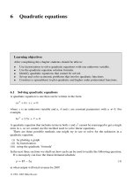
Consider the example of a firm that wishes to maximize output Q = f(K, L), with a fixed
budget M for purchasing inputs K and L at set prices PK and PL . This problem is illustrated
in Figure 11.1. The firm needs to find the combination of K and L that will allow it to reach
© 1993, 2003 Mike Rosser


K

M
PK

X
Q3
Q2
Q1
0

M
PL

L

Figure 11.1

the optimum point X which is on the highest possible isoquant within the budget constraint
with intercepts M/PK and M/PL .
To determine a solution for this type of economic resource allocation problem we have to

reformulate it as a mathematical constrained optimization problem. The following examples
suggest ways in which this can be done.

Example 11.1
A firm faces the production function Q = 12K 0.4 L0.4 and can buy the inputs K and L at
prices per unit of £40 and £5 respectively. If it has a budget of £800 what combination of K
and L should it use in order to produce the maximum possible output?
Solution
The problem is to maximize the function Q = 12K 0.4 L0.4 subject to the budget constraint
40K + 5L = 800

(1)

(In all problems in this chapter, it is assumed that each constraint ‘bites’; e.g. all the budget
is used in this example.)
The theory of the firm tells us that a firm is optimally allocating a fixed budget if the last £1
spent on each input adds the same amount to output, i.e. marginal product over price should
be equal for all inputs. This optimization condition can be written as
MPK
MPL
=
PK
PL
© 1993, 2003 Mike Rosser

(2)


The marginal products can be determined by partial differentiation:
∂Q

= 4.8K −0.6 L0.4
∂K
∂Q
MPL =
= 4.8K 0.4 L−0.6
∂L

MPK =

(3)
(4)

Substituting (3) and (4) and the given prices for PK and PL into (2)
4.8K −0.6 L0.4
4.8K 0.4 L−0.6
=
40
5
Dividing both sides by 4.8 and multiplying by 40 gives
K −0.6 L0.4 = 8K 0.4 L−0.6
Multiplying both sides by K 0.6 L0.6 gives
L = 8K

(5)

Substituting (5) for L into the budget constraint (1) gives
40K + 5(8K) = 800
40K + 40K = 800
80K = 800
Thus the optimal value of K is

K = 10
and, from (5), the optimal value of L is
L = 80
Note that although this method allows us to derive optimum values of K and L that satisfy
condition (2) above, it does not provide a check on whether this is a unique solution, i.e. there
is no second-order condition check. However, it may be assumed that in all the problems in
this section the objective function is maximized (or minimized depending on the question)
when the basic economic rules for an optimum are satisfied.
The above method is not the only way of tackling this problem by substitution. An alternative approach, explained below, is to encapsulate the constraint within the function to be
maximized, and then maximize this new objective function.

Example 11.1 (reworked)
Solution
From the budget constraint
40K + 5L = 800
5L = 800 − 40K

(1)

L = 160 − 8K

(2)

© 1993, 2003 Mike Rosser


Substituting (2) into the objective function Q = 12K 0.4 L0.4 gives
Q = 12K 0.4 (160 − 8K)0.4

(3)


We are now faced with the unconstrained optimization problem of finding the value of K that
maximizes the function (3) which has the budget constraint (1) ‘built in’ to it by substitution.
This requires us to set d Q/dK = 0. However, it is not straightforward to differentiate the
function in (3), and we must wait until further topics in calculus have been covered before
proceeding with this solution (see Chapter 12, Example 12.9).
To make sure that you understand the basic substitution method, we shall use it to tackle
another constrained maximization problem.

Example 11.2
A firm faces the production function Q = 20K 0.4 L0.6 . It can buy inputs K and L for £400 a
unit and £200 a unit respectively. What combination of L and K should be used to maximize
output if its input budget is constrained to £6,000?
Solution
∂Q
= 12K 0.4 L−0.4
∂L
Optimal input mix requires
MPL =

MPK =

∂Q
= 8K −0.6 L0.6
∂K

MPK
MPL
=
PL

PK
Therefore
8K −0.6 L0.6
12K 0.4 L−0.4
=
200
400
Cross multiplying gives
4,800K = 1,600L
3K = L
Substituting this result into the budget constraint
200L + 400K = 6,000
gives
200(3K) + 400K = 6,000
600K + 400K = 6,000
1,000K = 6,000
K=6
© 1993, 2003 Mike Rosser


Therefore
L = 3K = 18
The examples of constrained optimization considered so far have only involved output
maximization when a firm faces a Cobb–Douglas production function, but the same technique
can also be applied to other forms of production functions.

Example 11.3
A firm faces the production function
Q = 120L + 200K − L2 − 2K 2
for positive values of Q. It can buy L at £5 a unit and K at £8 a unit and has a budget of £70.

What is the maximum output it can produce?
Solution
∂Q
= 120 − 2L
∂L
For optimal input combination
MPL =

MPK =

∂Q
= 200 − 4K
∂K

MPL
MPK
=
PL
PK
Therefore, substituting MPK and MPL and the given input prices
120 − 2L
200 − 4K
=
5
8
8(120 − 2L) = 5(200 − 4K)
960 − 16L = 1,000 − 20K
20K = 40 + 16L
K = 2 + 0.8L


(1)

Substituting (1) into the budget constraint
5L + 8K = 70
gives
5L + 8(2 + 0.8L) = 70
5L + 16 + 6.4L = 70
11.4L = 54
L = 4.74
© 1993, 2003 Mike Rosser

(to 2 dp)


Substituting this result into (1)
K = 2 + 0.8(4.74) = 5.79
Therefore maximum output is
Q = 120L + 200K − L2 − 2K 2
= 120(4.74) + 200(5.79) − (4.74)2 − 2(5.79)2
= 1,637.28
This technique can also be applied to consumer theory, where utility is maximized subject
to a budget constraint.

Example 11.4
The utility a consumer derives from consuming the two goods A and B can be assumed to be
determined by the utility function U = 40A0.25 B 0.5 . If A costs £4 a unit and B costs £10 a
unit and the consumer’s income is £600, what combination of A and B will maximize utility?
Solution
The marginal utility of A is
MUA =


∂U
= 10A−0.75 B 0.5
∂A

The marginal utility of B is
MUB =

∂U
= 20A0.25 B −0.5
∂B

Consumer theory tells us that total utility will be maximized when the utility derived from
the last pound spent on each good is equal to the utility derived from the last pound spent on
any other good. This optimization rule can be expressed as
MUA
MUB
=
PA
PB
Therefore, substituting the above MU functions and the given prices of £4 and £10, this
condition becomes
10A−0.75 B 0.5
20A0.25 B −0.5
=
4
10
100B = 80A
B = 0.8A
Substituting (1) for B in the budget constraint

4A + 10B = 600
© 1993, 2003 Mike Rosser

(1)


gives
A + 10(0.8A) = 600
4A + 8A = 600
12A = 600
A = 50
Thus from (1)
B = 0.8(50) = 40
The substitution method can also be used for constrained minimization problems. If
output is given and a firm is required to minimize the cost of this output, then one variable
can be eliminated from the production function before it is substituted into the cost function
which is to be minimized.

Example 11.5
A firm operates with the production function Q = 4K 0.6 L0.4 and buys inputs K and L at
prices per unit of £40 and £15 respectively. What is the cheapest way of producing 600 units
of output?
Solution
The output constraint is
600 = 4K 0.6 L0.4
Therefore
150
= L0.4
K 0.6
150

K 0.6

2.5

=L

275,567.6
=L
K 1.5

(1)

The total cost of inputs, which is to be minimized, is
TC = 40K + 15L
Substituting (1) into (2) gives
TC = 40K + 15(275,567.6)K −1.5
© 1993, 2003 Mike Rosser

(2)


Differentiating and setting equal to zero to find a stationary point
dTC
= 40 − 22.5(275,567.6)K −2.5 = 0
dK
22.5(275,567.6)
40 =
K 2.5
22.5(275,567.6)
K 2.5 =

= 155,006.78
40
K = 119.16268

(3)

Substituting this value into (1) gives
L=

275,567.6
= 211.84478
(119.1628)1.5

This time we can check the second-order condition for minimization. Differentiating (3)
again gives
d2 TC
= (2.5)22.5(275,567.6)K −3.5 > 0 for any K > 0
dK 2
This confirms that these values minimize TC. We can also check that these values give 600
when substituted back into the production function.
Q = 4K 0.6 L0.4 = 4(119.16268)0.6 (211.84478)0.4 = 600
Thus cost minimization is achieved when K = 119.16 and L = 212.84 (to 2 dp) and so total
production costs will be
TC = 40(119.16) + 15(211.84) = £7,944

Test Yourself, Exercise 11.1
1.

2.


3.

4.

5.

If a firm has a budget of £378 what combination of K and L will maximize output
given the production function Q = 40K 0.6 L0.3 and prices for K and L of £20 per
unit and £6 per unit respectively?
A firm faces the production function Q = 6K 0.4 L0.5 . If it can buy input K at £32
a unit and input L at £8 a unit, what combination of L and K should it use to
maximize production if it is constrained by a fixed budget of £36,000?
A consumer spends all her income of £120 on the two goods A and B. Good A
costs £10 a unit and good B costs £15. What combination of A and B will she
purchase if her utility function is U = 4A0.5 B 0.5 ?
If a firm faces the production function Q = 4K 0.5 L0.5 , what is the maximum
output it can produce for a budget of £200? The prices of K and L are given as £4
per unit and £2 per unit respectively.
Make up your own constrained optimization problem for an objective function
with two independent variables and solve it using the substitution method.

© 1993, 2003 Mike Rosser


6.

A firm faces the production function Q = 2K 0.2 L0.6 and can buy L at £240 a unit
and K at £4 a unit.
(a)
(b)


7.

If it has a budget of £16,000 what combination of K and L should it use to
maximize output?
If it is given a target output of 40 units of Q what combination of K and L
should it use to minimize the cost of this output?

A firm has a budget of £1,140 and can buy inputs K and L at £3 and £8 respectively
a unit. Its output is determined by the production function
Q = 6K + 20L − 0.025K 2 − 0.05L2

8.

11.3

for positive values of Q. What is the maximum output it can produce?
A firm operates with the production function Q = 30K 0.4 L0.2 and buys inputs K
and L at £12 per unit and £5 per unit respectively. What is the cheapest way of
producing 750 units of output? (Work to nearest whole units of K and L.)

The Lagrange multiplier: constrained maximization
with two variables

The best way to explain how to use the Lagrange multiplier is with an example and so we
shall work through the problem in Example 11.1 from the last section using the Lagrange
multiplier method.
The firm is trying to maximize output Q = 12K 0.4 L0.4 subject to the budget constraint
40K + 5L = 800. The first step is to rearrange the budget constraint so that zero appears on
one side of the equality sign. Therefore

0 = 800 − 40K − 5L

(1)

We then write the ‘Lagrange equation’ or ‘Lagrangian’ in the form
G = (function to be optimized) + λ(constraint)
where G is just the value of the Lagrangian function and λ is known as the ‘Lagrange
multiplier’. (Do not worry about where these terms come from or what their actual values
are. They are just introduced to help the analysis. Note also that in other texts a ‘curly L’ is
often used to represent the Lagrange function. This can confuse students because economics
problems frequently involve labour, represented by L, as one of the variables in the function
to be optimized. This text therefore uses the notation ‘G’ to avoid this confusion. However,
if you are already accustomed to using the ‘curly L’ you can, of course, continue to use it
when answering problems yourself. What matters is whether you understand the analysis,
not what symbols you use.)
In this problem the Lagrange function is thus
G = 12K 0.4 L0.4 + λ(800 − 40K − 5L)
© 1993, 2003 Mike Rosser

(2)


Next, derive the partial derivatives of G with respect to K, L and λ and set them equal to
zero, i.e. find the stationary points of G that satisfy the first-order conditions for a maximum.
∂G
(3)
= 4.8K −0.6 L0.4 − 40λ = 0
∂K
∂G
(4)

= 4.8K 0.4 L−0.6 − 5λ = 0
∂L
∂G
= 800 − 40K − 5L = 0
(5)
∂λ
You will note that (5) is the same as the budget constraint (1). We now have a set of three linear
simultaneous equations in three unknowns to solve for K and L. The Lagrange multiplier λ
can be eliminated as, from (3),
0.12K −0.6 L0.4 = λ
and from (4)
0.96K 0.4 L−0.6 = λ
Therefore
0.12K −0.6 L0.4 = 0.96K 0.4 L−0.6
Multiplying both sides by K 0.6 L0.6 ,
0.12L = 0.96K
L = 8K

(6)

Substituting (6) into (5),
800 − 40K − 5(8K) = 0
800 = 80K
10 = K
Substituting back into (5),
800 − 40(10) − 5L = 0
400 = 5L
80 = L
These are the same values of K and L as those obtained by the substitution method. Thus,
the values of K and L that satisfy the first-order conditions for a maximum value of the

Lagrangian function G are the values that will maximize output subject to the given budget
constraint. We shall just accept this result without going into the proof of why this is so.
Strictly speaking we should now check the second-order conditions in the above problem
to be sure that we actually have a maximum rather than a minimum. These, however, are
rather complex, involving an examination of the function at and near the stationary points
found, and are discussed in the next section. For the time being you can assume that once
the stationary points of a Lagrangian function have been found the second-order conditions
for a maximum will automatically be met. Some more examples are worked through so that
you can become familiar with this method.
© 1993, 2003 Mike Rosser


Example 11.6
A firm can buy two inputs K and L at £18 per unit and £8 per unit respectively and faces
the production function Q = 24K 0.6 L0.3 . What is the maximum output it can produce for a
budget of £50,000? (Work to nearest whole units of K, L and Q.)
Solution
The budget constraint is 50,000 − 18K − 8L = 0 and the function to be maximized is
Q = 24K 0.6 L0.3 . The Lagrangian for this problem is therefore
G = 24K 0.6 L0.3 + λ(50,000 − 18K − 8L)
Partially differentiating to find the stationary points of G gives
∂G
= 14.4K −0.4 L0.3 − 18λ = 0
∂K
14.4L0.3
=λ
18K 0.4
∂G
= 7.2K 0.6 L−0.7 − 8λ = 0
∂L

7.2K 0.6
=λ
8L0.7
∂G
= 50,000 − 18K − 8L = 0
∂λ

(1)

(2)
(3)

Setting (1) equal to (2) to eliminate λ
7.2K 0.6
14.4L0.3
=
18K 0.4
8L0.7
115.2L = 129.6K
L = 1.125K

(4)

Substituting (4) into (3)
50,000 − 18K − 8(1.125K) = 0
50,000 − 18K − 9K = 0
50,000 = 27K
1,851.8519 = K

(5)


Substituting (5) into (4)
L = 1.125(1,851.8519) = 2,083.3334
Thus, to the nearest whole unit, optimum values of K and L are 1,852 and 2,083 respectively.
© 1993, 2003 Mike Rosser


We can check that when these whole values of K and L are used the total cost will be
TC = 18K + 8L = 18(1,852) + 8(2,083) = 33,336 + 16,664 = £50,000
and so the budget constraint is satisfied. The actual maximum output level will be
Q = 24K 0.6 L0.3 = 24(1,852)0.6 (2,083)0.3 = 21,697 units
Although the same mathematical method can be used for various economic applications,
you must learn to use your knowledge of economics to set up the mathematical problem in
the first place. The example below demonstrates another application of the Lagrange method.

Example 11.7
A consumer has the utility function U = 40A0.5 B 0.5 . The prices of the two goods A and B
are initially £20 and £5 per unit respectively, and the consumer’s income is £600. The price
of A then falls to £10. Work out the income and substitution effects of this price change on
the amount of A consumed using Hicks’s method and say whether A and B are normal or
inferior goods.
Solution
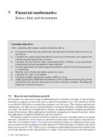
To help solve this problem the relevant budget schedules and indifference curves are illustrated
in Figure 11.2, although the indifference curves are not accurately drawn to scale. The original
optimum is at X. The price fall for A causes the budget line to become flatter and swing round,
giving a new equilibrium at Y.
Hicks’s method for splitting the total change in A into its income and substitution effects
requires one to draw a ‘ghost’ budget line parallel to the new budget line (reflecting the new

B

120

60

X

Y
H

42.4

II
I

0

15 21.2

Figure 11.2
© 1993, 2003 Mike Rosser

30

60

A


relative prices) but tangential to the original indifference curve. This is shown by the broken
line tangential to indifference curve I at H. From X to H is the substitution effect and from H to

Y is the income effect of the price change. This problem requires us to find the corresponding
values of A and B for the three tangency points X, Y and H and then to comment on the
direction of these changes.
The original equilibrium is the combination of A and B that maximizes the utility function
U = 40A0.5 B 0.5 subject to the budget constraint 600 = 20A + 5B. These values of A and
B can be found by deriving the stationary points of the Lagrange function
G = 40A0.5 B 0.5 + λ(600 − 20A − 5B)
Thus
∂G
= 20A−0.5 B 0.5 − 20λ = 0
∂A
∂G
= 20A0.5 B −0.5 − 5λ = 0
∂B
∂G
= 600 − 20A − 5B = 0
∂λ

giving A−0.5 B 0.5 = λ
giving

4A0.5 B −0.5 = λ

(1)
(2)
(3)

Setting (1) equal to (2)
A−0.5 B 0.5 = 4A0.5 B −0.5
B = 4A


(4)

Substituting (4) into (3)
600 − 20A − 5(4A) = 0
600 = 40A
15 = A
Substituting this value into (4)
B = 4(15) = 60
Thus, A = 15 and B = 60 at the original equilibrium at X.
When the price of A falls to 10, the budget constraint becomes
600 = 10A + 5B
and so the new Lagrange function is
G = 40A0.5 B 0.5 + λ(600 − 10A − 5B)
New stationary points will be where
∂G
= 20A−0.5 B 0.5 − 10λ = 0
∂A
∂G
= 20A0.5 B −0.5 − 5λ = 0
∂B
∂G
= 600 − 10A − 5B = 0
∂λ
© 1993, 2003 Mike Rosser

giving

2A−0.5 B 0.5 = λ


(5)

giving

4A0.5 B −0.5 = λ

(6)
(7)


Setting (5) equal to (6)
2A−0.5 B 0.5 = 4A0.5 B −0.5
B = 2A

(8)

Substituting (8) into (7)
600 − 10A − 5(2A) = 0
600 = 20A
30 = A
Substituting this value into (8) gives
B = 2(30) = 60.
Thus, the total effect of the price change is to increase consumption of A from 15 to 30 units
and leave consumption of B unchanged at 60.
There are several ways of finding the values of A and B that correspond to point H. We
know that H is on the same indifference curve as point X, and therefore the utility function
will take the same value at both points. We can find the value of utility at X where A = 15
and B = 60. This will be
U = 40A0.5 B 0.5 = 40(15)0.5 (60)0.5 = 40(900)0.5 = 40(30) = 1,200
Thus, at any point on the indifference curve I

40A0.5 B 0.5 = 1,200
B 0.5 = 30A−0.5
B = 900A−1

(9)

The slope of indifference curve I will therefore be
dB
= −900A−2
dA

(10)

At point X, the indifference curve I is tangential to the new budget line whose slope will be
−PA
−10
=
= −2
PB
5
Therefore, from (10) and (11)
−900A−2 = −2
450 = A2
21.2132 = A
Substituting this value into (9)
B = 900(21.2132)−1 = 42.4264
© 1993, 2003 Mike Rosser

(11)



Thus the substitution effect of A’s price fall, from X to H, increases consumption of A from
15 to 21.2 units and decreases consumption of B from 60 to 42.4 units. This effect is negative
(i.e. quantity rises when price falls) in line with standard consumer theory.
The income effect, from H to Y, increases consumption of A from 21.2 to 30 units and
also increases consumption of B from 42.4 back to its original 60 unit level. As both income
effects are positive, both A and B must be normal goods.

Test Yourself, Exercise 11.2
Use the Lagrange method to answer questions 1, 2, 3, 4, 6(a) and 7 from Test
Yourself, Exercise 11.1.

11.4

The Lagrange multiplier: second-order conditions

Inasmuch as it involves setting the first derivatives of the objective function equal to zero,
the Lagrange method of solving constrained optimization problems is similar to the method
of solving unconstrained optimization problems involving functions of several variables that
was explained in Chapter 10. However, one cannot simply apply the same set of second-order
conditions to check for a maximum or minimum because of the special role that the Lagrange
multiplier takes. The mathematics required to prove why this is so, and to explain what
additional second-order conditions are necessary for a Lagrangian function to be a maximum
or minimum, becomes rather complex. We shall therefore just look at an intuitive explanation
of what these conditions involve here. The use of matrix algebra to check second-order
conditions in constrained optimization problems will then be explained later in Chapter 15.
First, we shall consider the conditions for a maximum. If we assume that a function has two
independent variables then both the function to be maximized, f(A, B), and the constraint
could take on several possible forms, as illustrated in Figure 11.3. These diagrams are all
constructed on the same basis as isoquant maps. Thus the lines I, II and III represent different

levels of the objective function with its value increasing as one moves away from the origin.
In Figure 11.3(a), the objective function is convex to the origin and the constraint CD is
linear. Maximization of the objective function occurs at the tangency point T.

(a) B

(b) B

C

C

T

II

T

I

C III
R

I

III

III
II


0

(c) B

II

T

S

D

I
D

Figure 11.3
© 1993, 2003 Mike Rosser

A

0

D

A

0

A



In Figure 11.3(b), the objective function is concave to the origin and so it is maximized
subject to the linear constraint CD at the corner point C. Thus the tangency point T does not
determine the maximum value.
In Figure 11.3(c), the objective function is convex to the origin but the constraint CD is
non-linear and more sharply curved than the objective function. Thus the tangency point T
is not the maximum value. Higher values of the objective function can be found at points R
and S, for example.
From the above examples we can see that, for the two-variable case, a linear constraint
and an objective function that is convex to the origin will ensure maximization at the point
of tangency. In other cases, tangency may not ensure maximization. If a problem involves
the maximization of production subject to a linear budget constraint this means that output
is maximized where the slope of the isoquant is equal to the slope of the budget constraint.
We have already seen in Chapter 10 how a Cobb–Douglas production function in the form
Q = AK α Lβ will correspond to a set of isoquants which continually decline and become
flatter as L is increased, i.e. are convex to the origin. Thus in any constrained optimization
problem where one is attempting to maximize a production function in the Cobb–Douglas
format subject to a linear budget constraint, the input combination that satisfies the first-order
conditions will be a maximum.
If the Lagrangian represents other concepts with similar shaped functions and constraints,
such as utility, the same conditions apply. In all such cases, one assumes that the independent
variables in the objective function must take positive values and so any negative mathematical
solutions can be disregarded.
Although we cannot illustrate functions with more than two variables diagrammatically, the
same basic principles apply when one is attempting to maximize a function with three or more
variables subject to a linear constraint. Thus any Cobb–Douglas production function with
more than two inputs will be at a maximum, subject to a specified linear budget constraint,
when the first-order conditions for optimization of the relevant Lagrange equation are met. For
the purpose of answering the problems in this Chapter, and for most constrained maximization
problems that you will encounter in a first-year economics course, it can be assumed that

the stationary points of the Lagrange function will satisfy the second-order conditions for a
maximum.
The properties of the objective function and constraint that guarantee that a Lagrange
function is minimized when first-order conditions are met are the reverse of the properties
required for a maximum, i.e. the objective function must be linear and the constraint must
be convex to the origin. Thus if one is required to find values of K and L that minimize a
budget function in the form
TC = PK K + PL L
subject to a given output Q∗ being produced via the production function Q = AK α Lβ , then
the corresponding Lagrange function is
G = PK K + PL L + λ(Q∗ − AK α Lβ )
and the values of K and L which satisfy the first-order conditions
∂G
=0
∂K

∂G
=0
∂L

will also satisfy second-order conditions for a minimum.
© 1993, 2003 Mike Rosser


If you refer back to Figure 11.3(a) you can see the rationale for this rule in the two-input
case. If input prices are given and one is trying to minimize the cost of the output represented
by isoquant II, then one needs to find the budget constraint with slope equal to the negative
of the price ratio which is nearest the origin and still goes through this isoquant. The linear
objective function and the constraint convex to the origin guarantee that this will be at the
tangency point T. Some examples of minimization problems that use this rule are given in

the next section.
To conclude this section, let us reiterate what we have learned about second-order conditions and Lagrangians. When the objective function is in the Cobb–Douglas format and the
constraint is linear, then the second-order conditions for a maximum are met at the stationary
points of the Lagrange function. This rule is reversed for minimization.

11.5

Constrained minimization using the Lagrange multiplier

As was explained in Section 11.4, the same principles used to construct a Lagrange function
for a constrained maximization problem are used to construct a Lagrange function for a
constrained minimization problem. The difference is that the components of the function
are reversed, as is shown in the following examples. In all these cases the constraints and
objective function take formats which guarantee that second-order conditions for a minimum
are met.

Example 11.8
A firm operates with the production function Q = 4K 0.6 L0.5 and can buy K at £15 a unit
and L at £8 a unit. What input combination will minimize the cost of producing 200 units of
output?

Solution
The output constraint is 200 = 4K 0.6 L0.5 and the objective function to be minimized is the
total cost function TC = 15K + 8L. The corresponding Lagrangian function is therefore
G = 15K + 8L + λ(200 − 4K 0.6 L0.5 )
Partially differentiating G and setting equal to zero, first-order conditions require
∂G
= 15 − λ2.4K −0.4 L0.5 = 0 giving
∂K
∂G

= 8 − λ2K 0.6 L−0.5 = 0
giving
∂L
∂G
= 200 − 4K 0.6 L0.5 = 0
∂λ
© 1993, 2003 Mike Rosser

15K 0.4
=λ
2.4L0.5
4L0.5
=λ
K 0.6

(1)
(2)
(3)


Setting (1) equal to (2) to eliminate λ
15K 0.4
4L0.5
= 0.6
2.4L0.5
K
15K = 9.6L
1.5625K = L

(4)


Substituting (4) into (3)
200 − 4K 0.6 (1.5625K)0.5 = 0
200 = 4K 0.6 (1.5625)0.5 K 0.5
200
= K 1.1
4(1.5625)0.5
40 = K 1.1
√
1.1
K = 40 = 28.603434
Substituting this value into (4)
1.5625(28.603434) = L
44.692866 = L
Thus the optimal input combination is 28.6 units of K plus 44.7 units of L (to 1 dp). We can
check that these input values correspond to the given output level by substituting them back
into the production function. Thus
Q = 4K 0.6 L0.5 = 4(28.6)0.6 (44.7)0.5 = 200
which is correct, allowing for rounding error. The actual cost entailed will be
TC = 15K + 8L = 15(28.6) + 8(44.7) = £786.60

Example 11.9
The prices of inputs K and L are given as £12 per unit and £3 per unit respectively, and a firm
operates with the production function Q = 25K 0.5 L0.5 .
(i) What is the minimum cost of producing 1,250 units of output?
(ii) Demonstrate that the maximum output that can be produced for this budget will be the
1,250 units specified in (i) above.
Solution
This question essentially asks us to demonstrate that the constrained maximization and
minimization methods give consistent answers.

(i) The output constraint is that
1,250 = 25K 0.5 L0.5
© 1993, 2003 Mike Rosser


The objective function to be minimized is the cost function
TC = 12K + 3L
The corresponding Lagrange function is therefore
G = 12K + 3L + λ(1,250 − 25K 0.5 L0.5 )
First-order conditions require
∂G
= 12 − λ12.5K −0.5 L0.5 = 0
∂K
∂G
= 3 − λ12.5K 0.5 L−0.5 = 0
∂L
∂G
= 1,250 − 25K 0.5 L0.5 = 0
∂λ

giving
giving

12K 0.5
=λ
12.5L0.5
3L0.5
=λ
12.5K 0.5


(1)
(2)
(3)

Setting (1) equal to (2)
3L0.5
12K 0.5
=
12.5L0.5
12.5K 0.5
4K = L

(4)

Substituting (4) into (3)
1,250 − 25K 0.5 (4K)0.5 = 0
1,250 = 25K 0.5 (4)0.5 K 0.5
1,250 = 50K
25 = K
Substituting this value into (4)
4(25) = L
100 = L
When these optimum values of K and L are used the actual minimum cost will be
TC = 12K + 3L = 12(25) + 3(100) = 300 + 300 = £600
(ii) This part of the question requires us to find the values of K and L that will maximize
output subject to a budget of £600, i.e. the answer to (i) above. The objective function to
be maximized is therefore Q = 25K 0.5 L0.5 and the constraint is 12K + 3L = 600. The
corresponding Lagrange equation is thus
G = 25K 0.5 L0.5 + λ(600 − 12K − 3L)
© 1993, 2003 Mike Rosser



First-order conditions require
∂G
= 12.5K −0.5 L0.5 − 12λ = 0
∂K
∂G
= 12.5K 0.5 L−0.5 − 3λ = 0
∂L
∂G
= 600 − 12K − 3L = 0
∂λ

giving
giving

12.5L0.5
=λ
12K 0.5
12.5K 0.5
=λ
3L0.5

(5)
(6)
(7)

Setting (5) equal to (6)
12.5K 0.5
12.5L0.5

=
12K 0.5
3L0.5
3L = 12K
L = 4K

(8)

Substituting (8) into (7)
600 − 12K − 3(4K) = 0
600 − 12K − 12K = 0
600 = 24K
25 = K
Substituting this value into (8) L = 4(25) = 100
These are the same optimum values of K and L that were found in part (i) above. The
actual output produced by 25 of K plus 100 of L will be
Q = 25K 0.5 L0.5 = 25(25)0.5 (100)0.5 = 1,250
which checks out with the amount specified in the question.
Although most of the examples of constrained optimization presented in this chapter are
concerned with a firm’s output and costs, or a consumer’s utility level and income, the
Lagrange method can be applied to other areas of economics. For instance, in environmental
economics one may wish to find the cheapest way of securing a given level of environmental
cleanliness.

Example 11.10
Assume that there are two sources of pollution into a lake. The local water authority can clean
up the discharges and reduce pollution levels from these sources but there are, of course, costs
involved. The damage effects of each pollution source are measured on a ‘pollution scale’.
The lower the pollution level the greater the cost of achieving it, as is shown by the cost
schedules for cleaning up the two pollution sources:

0.5
Z1 = 478 − 2C1

© 1993, 2003 Mike Rosser

0.5
and Z2 = 600 − 3C2


where Z1 and Z2 are pollution levels and C1 and C2 are expenditure levels (in £000s) on
reducing pollution.
To secure an acceptable level of water purity in the lake the water authority’s objective is
to reduce the total pollution level to 1,000 by the cheapest method. How can it do this?
Solution
This can be formulated as a constrained optimization problem where the constraint is the
total amount of pollution Z1 + Z2 = 1000 and the objective function to be minimized is the
cost of pollution control TC = C1 + C2 . Thus the Lagrange function is
G = C1 + C2 + λ(1,000 − Z1 − Z2 )
Substituting in the cost functions for Z1 and Z2 , this becomes
0.5
0.5
G = C1 + C2 + λ[1,000 − (478 − 2C1 ) − (600 − 3C2 )]
0.5
0.5
G = C1 + C2 + λ(−78 + 2C1 + 3C2 )

First-order conditions require
∂G
−0.5
= 1 + λC1

=0
∂C1
∂G
−0.5
= 1 + λ1.5C2
=0
∂C2
∂G
0.5
0.5
= −78 + 2C1 + 3C2 = 0
∂λ

giving

0.5
λ = −C1

(1)

giving

λ=

0.5
−C2
1.5

(2)
(3)


Equating (1) and (2)
0.5
−C1 =

0.5
−C2
1.5

0.5
0.5
1.5C1 = C2

(4)

Substituting (4) into (3)
0.5
0.5
−78 + 2C1 + 3(1.5C1 ) = 0
0.5
0.5
2C1 + 4.5C1 = 78
0.5
6.5C1 = 78
0.5
C1 = 12

C1 = 144
Substituting (5) into (4)
0.5

C2 = 1.5(12) = 18

C2 = 324
© 1993, 2003 Mike Rosser

(5)


We can use these optimum pollution control expenditure amounts to check the total pollution
level:
0.5
0.5
Z1 + Z2 = [(478 − 2C1 ) + (600 − 3C2 )]

= 478 − 2(12) + 600 − 3(18)
= 1,000
which is the required level. Thus the water authority should spend £144,000 on reducing the
first pollution source and £324,000 on reducing the second source.

Test Yourself, Exercise 11.3
1.
2.

3.

4.

11.6

Use the Lagrange multiplier to answer Questions 6(b) and 8 from Test Yourself,

Exercise 11.1.
What is the cheapest way of producing 850 units of output if a firm operates with
the production function Q = 30K 0.5 L0.5 and can buy input K at £75 a unit and L
at £40 a unit?
Two pollution sources can be cleaned up if money is spent on them according to
0.5
0.5
the functions Z1 = 780 − 12C1 and Z2 = 600 − 8C2 where Z1 and Z2 are
the pollution levels from the two sources and C1 and C2 are expenditure levels
(in £000s) on pollution reduction. What is the cheapest way of reducing the total
pollution level from 1,380, which is the level it would be without any controls, to
1,000?
A firm buys inputs K and L at £70 a unit and £30 a unit respectively and faces the
production function Q = 40K 0.5 L0.5 . What is the cheapest way it can produce an
output of 500 units?

Constrained optimization with more than two variables

The same procedures that were used for two-variable problems are also used for applying the
Lagrange method to constrained optimization problems with three or more variables. The
only difference is that one has a more complex set of simultaneous equations to solve for
the optimum values that satisfy the first-order conditions. Although some of these sets of
equations may initially look rather awkward to work with, they can usually be greatly simplified and solutions can be found by basic algebra, as the following examples show. As
with the two-variable problems, it is assumed that second-order conditions for a maximum
(or minimum) are satisfied at stationary points of the Lagrange function in the problems set
out here.

Example 11.11
A firm has a budget of £300 to spend on the three inputs x, y and z whose prices per unit are
£4, £1 and £6 respectively. What combination of x, y and z should it employ to maximize

output if it faces the production function Q = 24x 0.3 y 0.2 z0.3 ?
© 1993, 2003 Mike Rosser


Solution
The budget constraint is
300 − 4x − y − 6z = 0
and the objective function to be maximized is
Q = 24x 0.3 y 0.2 z0.3
Thus the Lagrange function is
G = 24x 0.3 y 0.2 z0.3 + λ(300 − 4x − y − 6z)
Differentiating with respect to each variable and setting equal to zero gives
∂G
∂x
∂G
∂y
∂G
∂z
∂G
∂λ

= 7.2x −0.7 y 0.2 z0.3 − 4λ = 0

λ = 1.8x −0.7 y 0.2 z0.3

(1)

= 4.8x 0.3 y −0.8 z0.3 − λ = 0

λ = 4.8x 0.3 y −0.8 z0.3


(2)

= 7.2x 0.3 y 0.2 z−0.7 − 6λ = 0

λ = 1.2x 0.3 y 0.2 z−0.7

(3)

= 300 − 4x − y − 6z = 0

(4)

A simultaneous three-linear-equation system in the three unknowns x, y and z can now be
set up if λ is eliminated. There are several ways in which this can be done. In the method
used below we set (1) and then (3) equal to (2) to eliminate x and z and then substitute into
(4) to solve for y. Whichever method is used, the point of the exercise is to arrive at functions
for any two of the unknown variables in terms of the remaining third variable.
Thus, setting (1) equal to (2)
1.8x −0.7 y 0.2 z0.3 = 4.8x 0.3 y −0.8 z0.3
Multiplying both sides by x 0.7 y 0.8 and dividing by z0.3 gives
1.8y = 4.8x
0.375y = x

(5)

We have now eliminated z and obtained a function for x in terms of y. Next we need to
eliminate x and obtain a function for z in terms of y. To do this we set (2) equal to (3), giving
4.8x 0.3 y −0.8 z0.3 = 1.2x 0.3 y 0.2 z−0.7
Multiplying through by z0.7 y 0.8 and dividing by x 0.3 gives

4.8z = 1.2y
z = 0.25y
© 1993, 2003 Mike Rosser

(6)


Substituting (5) and (6) into the budget constraint (4)
300 − 4(0.375y) − y − 6(0.25y) = 0
300 − 1.5y − y − 1.5y = 0
300 = 4y
75 = y
Therefore, from (5)
x = 0.375(75) = 28.125
and from (6)
z = 0.25(75) = 18.75

If these optimal values of x, y and z are used then the maximum output will be
Q = 24x 0.3 y 0.2 z0.3 = 24(28.125)0.3 (75)0.2 (18.75)0.3 = 373.1 units.

Example 11.12
A firm uses the three inputs K, L and R to manufacture good Q and faces the production
function
Q = 50K 0.4 L0.2 R 0.2
It has a budget of £24,000 and can buy K, L and R at £80, £12 and £10 respectively per unit.
What combination of inputs will maximize its output?
Solution
The objective function to be maximized is Q = 50K 0.4 L0.2 R 0.2 and the budget constraint is
24,000 − 80K − 12L − 10R = 0
Thus the Lagrange equation is

G = 50K 0.4 L0.2 R 0.2 + λ(24,000 − 80K − 12L − 10R)
Differentiating
∂G
∂K
∂G
∂L
∂G
∂R
∂G
∂λ

= 20K −0.6 L0.2 R 0.2 − 80λ = 0

λ = 0.25K −0.6 L0.2 R 0.2

= 10K 0.4 L−0.8 R 0.2 − 12λ = 0

λ=

= 10K 0.4 L0.2 R −0.8 − 10λ = 0

λ = K 0.4 L0.2 R −0.8

= 24,000 − 80K − 12L − 10R = 0

© 1993, 2003 Mike Rosser

10 0.4 −0.8 0.2
K L
R

12

(1)
(2)
(3)
(4)


Equating (1) and (2) to eliminate R
10 0.4 −0.8 0.2
R
K L
12
3L = 10K

0.25K −0.6 L0.2 R 0.2 =

0.3L = K

(5)

Equating (2) and (3) to eliminate K and get R in terms of L
10 0.4 −0.8 0.2
R = K 0.4 L0.2 R −0.8
K L
12
10R = 12L
R = 1.2L

(6)


Substituting (5) and (6) into (4)
24,000 − 80(0.3L) − 12L − 10(1.2L) = 0
24,000 = 24L + 12L + 12L
24,000 = 48L
500 = L
Substituting this value for L into (5) and (6)
K = 0.3(500) = 150

R = 1.2(500) = 600

Using these optimal values for K, L and R, the firm’s maximum output will be
Q = 50K 0.4 L0.2 R 0.2 = 50(150)0.4 (500)0.2 (600)0.2 = 4,622 units

Example 11.13
A firm buys the four inputs K, L, R and M at per-unit prices of £50, £30, £25 and £20
respectively and operates with the production function
Q = 160K 0.3 L0.25 R 0.2 M 0.25
What is the maximum output it can make for a total cost of £30,000?
Solution
The relevant Lagrange function is
G = 160K 0.3 L0.25 R 0.2 M 0.25 + λ(30,000 − 50K − 30L − 25R − 20M)
© 1993, 2003 Mike Rosser